Fun with Filters and Frequencies!

CS180: Intro to Computer Vision and Computational Photography

Srinidhi Raghavendran

Overview

In this project, we explore the world of image filtering and frequency analysis to gain insight into image manipulation and transformations. The goal is to understand how convolution filters work and how different frequency manipulations affect images.

Part 1: Fun with Filters

1.1: Finite Difference Operator

Using finite difference operators to compute the image gradients in the x and y directions helps identify the edges in an image.

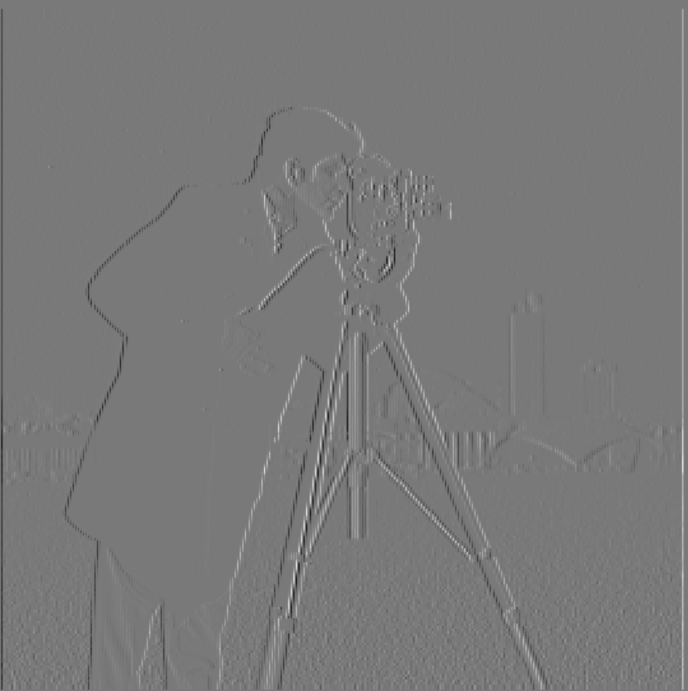
Gradient dx

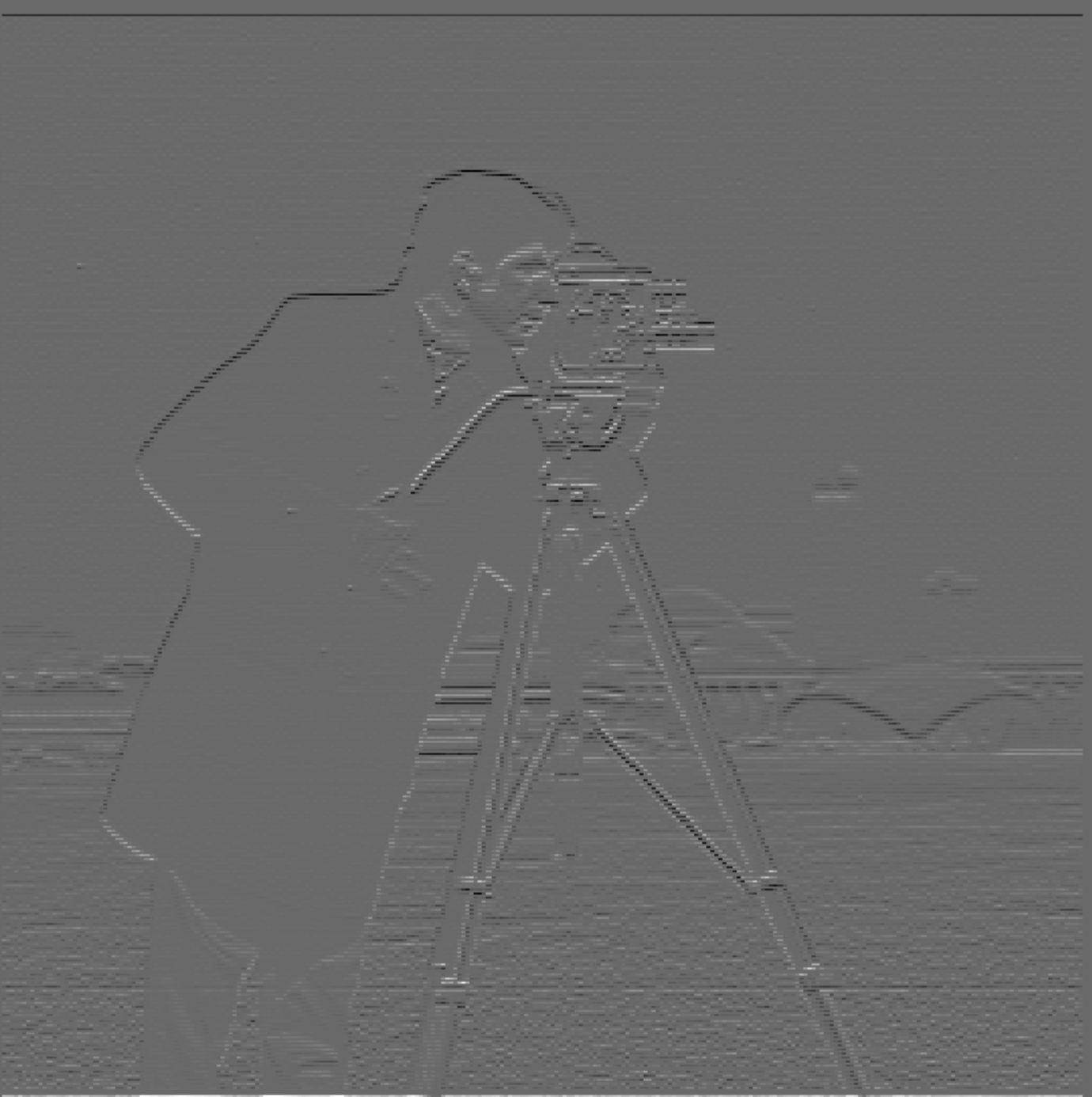
Gradient dy

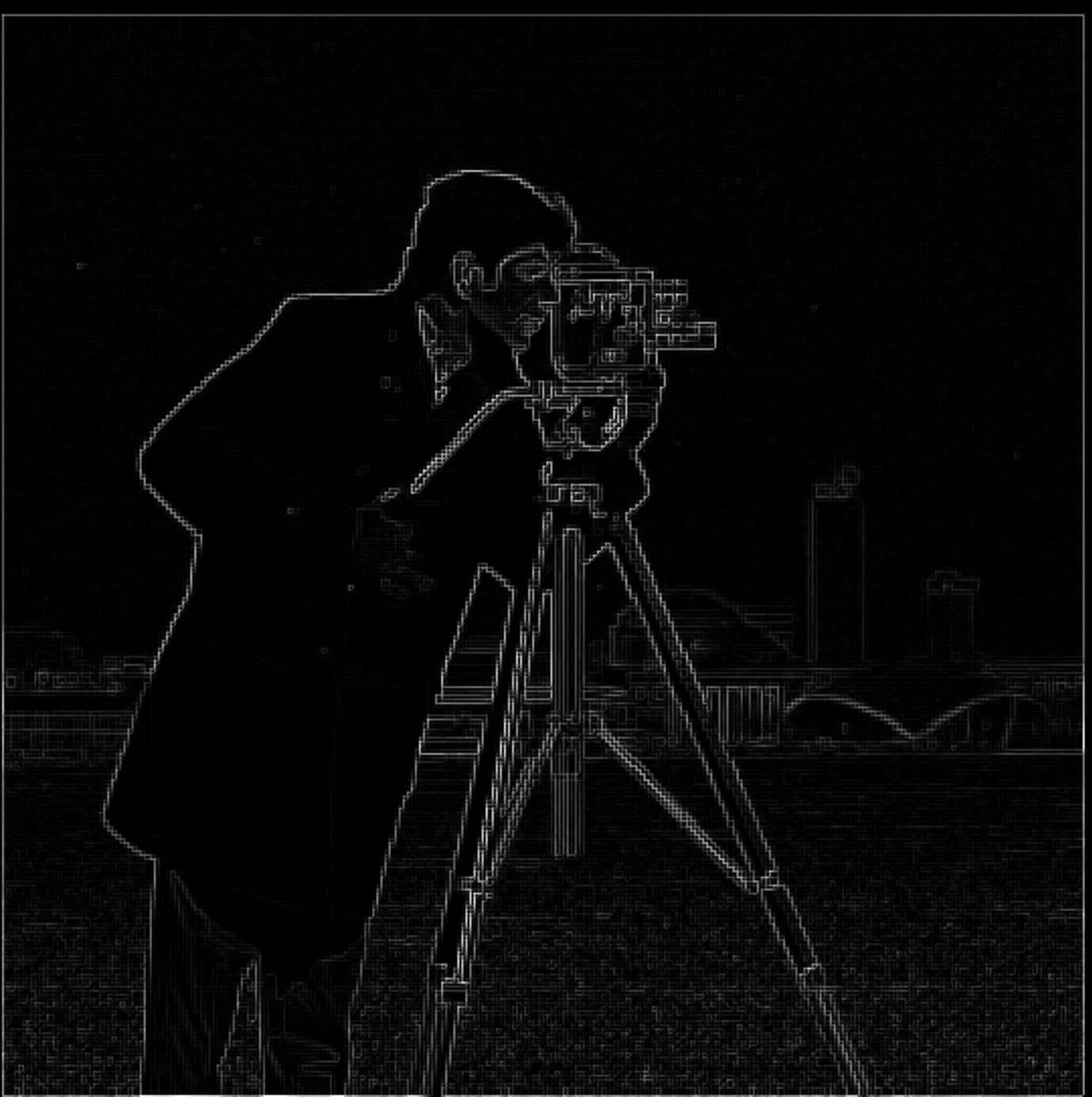
Gradient Magnitude Image

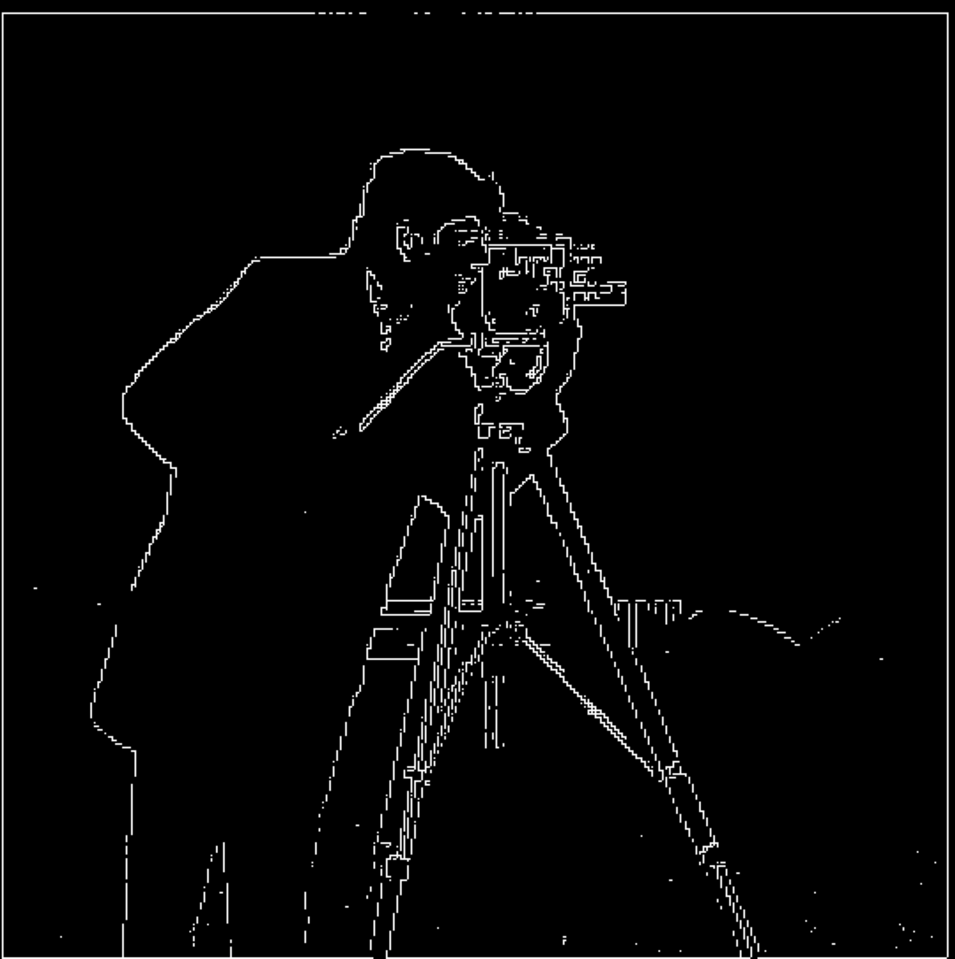
Binarized Edge Image

1.2: Derivative of Gaussian (DoG) Filter

We noted that the results with just the difference operator were rather noisy. Luckily, we have a smoothing operator handy: the Gaussian filter.

First, we create a blurred version of the original image by convolving it with a Gaussian filter (G) and repeat the procedure in the previous part. To create a 2D Gaussian filter, we use the cv2.getGaussianKernel() function to generate a 1D Gaussian, and then take the outer product with its transpose to form a 2D Gaussian kernel.

By comparing the results, we notice a significant reduction in noise. This is because the Gaussian filter smooths out high-frequency variations.

Original Image

Blurred Image (Gaussian)

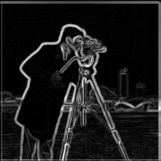
Gradient Magnitude (Gaussian)

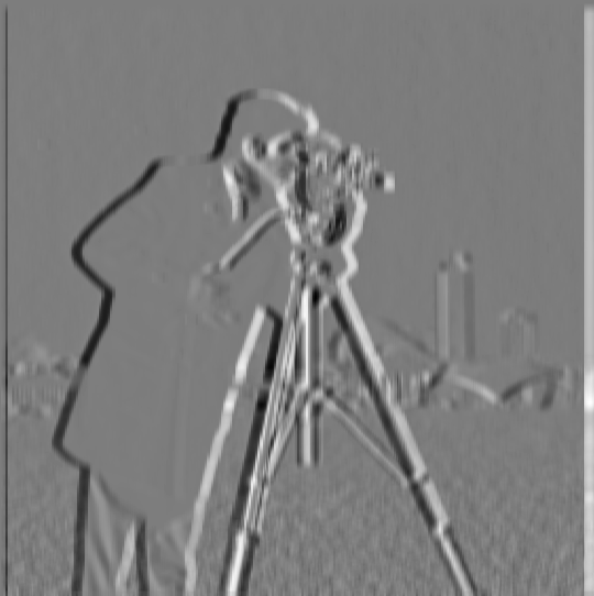
DoG Filter (X-Direction)

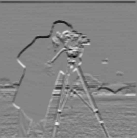
DoG Filter (Y-Direction)

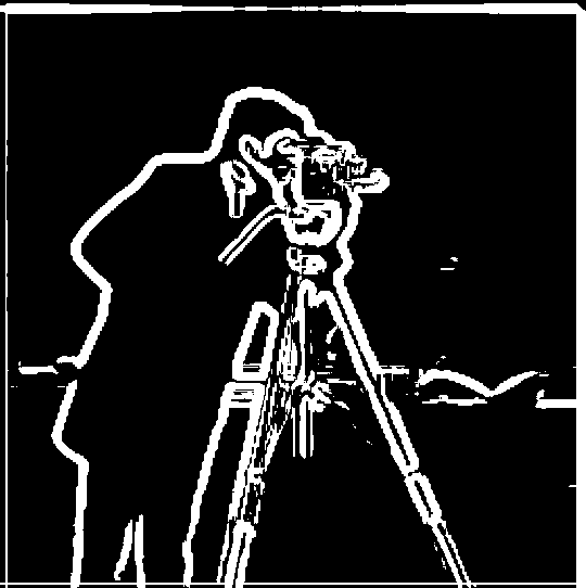
Binarized Edge Image

By using the Derivative of Gaussian (DoG) filters in both x and y directions, we can effectively highlight the edges and reduce noise. This results in a much cleaner edge detection compared to using just the finite difference operator.

Next, we want to demonstrate the commutative property of convolution. Instead of blurring the image first, we convolve the Gaussian filter (G) with the derivative operators (D_x and D_y) to create the Derivative of Gaussian (DoG) filters. We then apply these DoG filters directly to the original image. This should yield the same result as the previous method.

Unfortunately, even though I followed the expected steps for this part, the results did not align with those from the previous method. This discrepancy might be due to the effect of boundary conditions and padding, which can disrupt the commutative property in a finite image. In theory, applying the DoG filters to the original image should have yielded the same edge detection as applying the Gaussian followed by the derivatives. However, due to the padding artifacts introduced at the image boundaries, the results were not as expected.

This highlights an important consideration when dealing with discrete convolutions: while the commutative property holds true in continuous domains, finite images and padding can introduce variations that disrupt this behavior. This is a good lesson for the future that rather than just blindly assuming it doesn't work, we understand and account for these factors in the future.

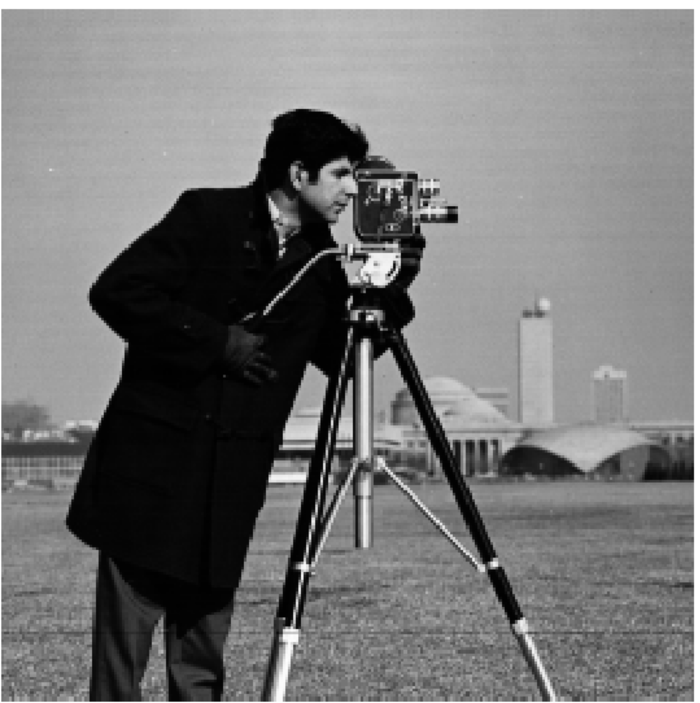
Original Image

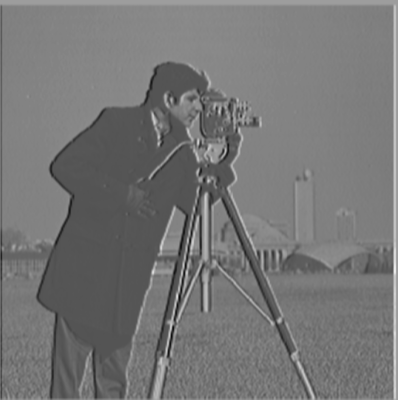
DoG Filter (X-Direction)

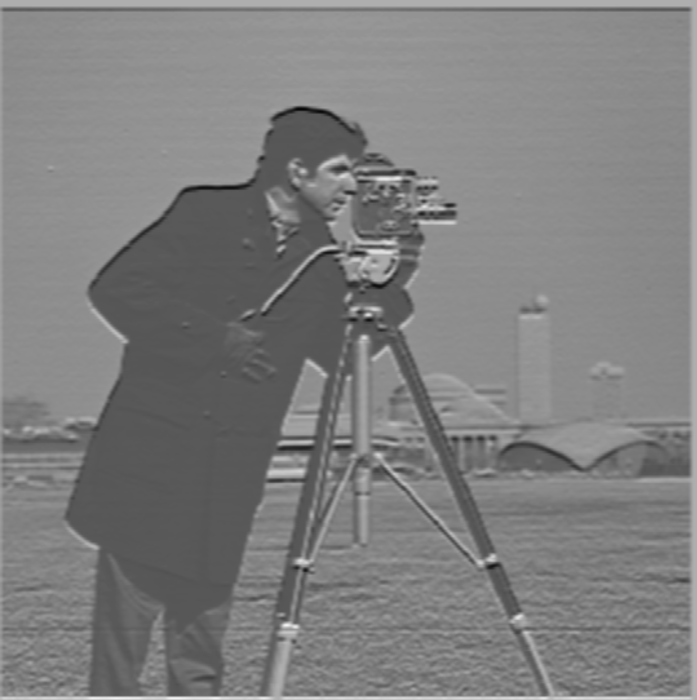
DoG Filter (Y-Direction)

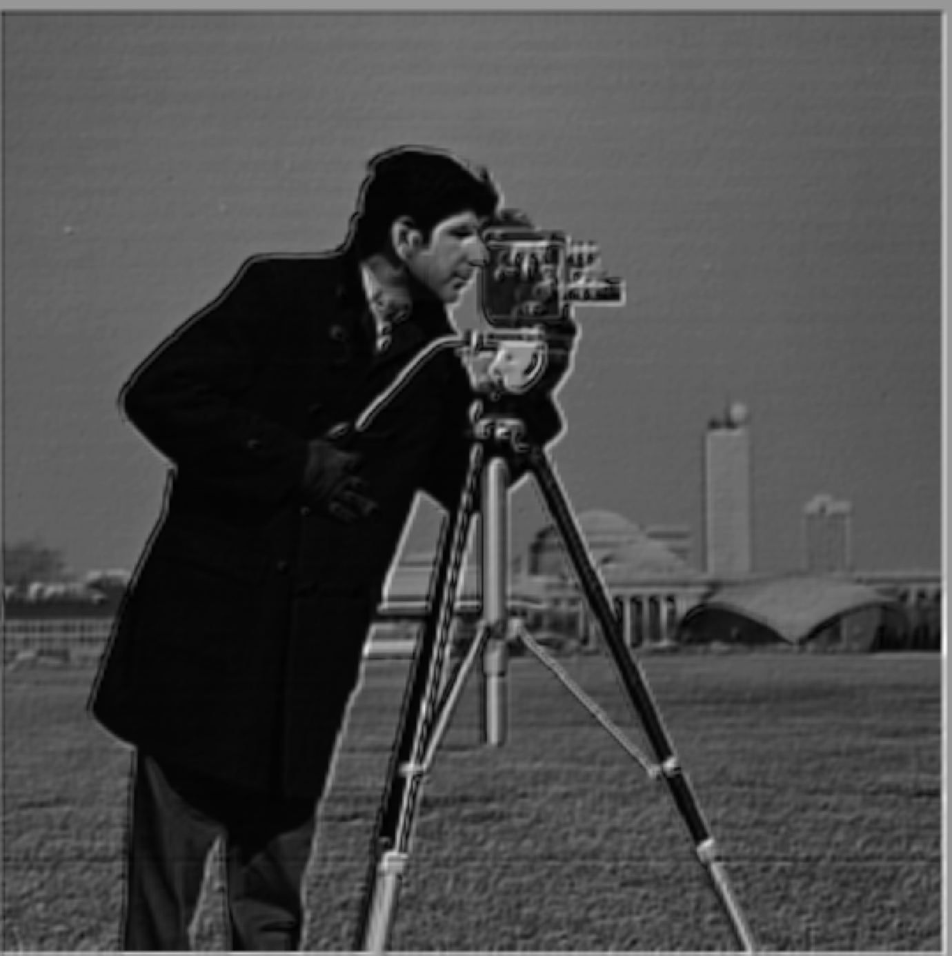
Gradient Magnitude (DoG)

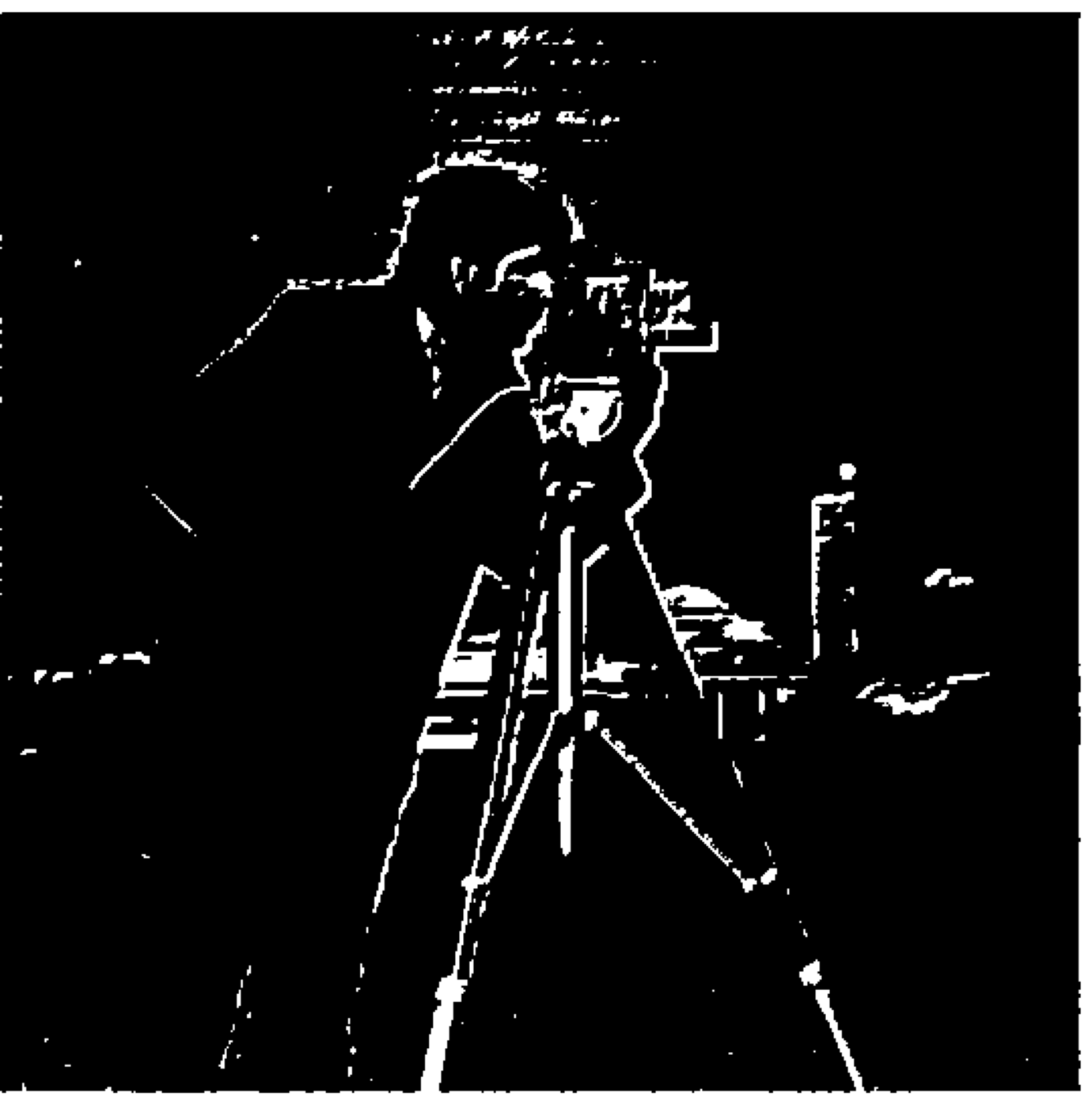
Binarized Edge Image (DoG)

Despite following the expected steps, the results obtained from applying the DoG filters directly to the original image did not perfectly match those from the previous method of blurring first and then applying the finite difference operators. This discrepancy can be attributed to the effects of padding and boundary conditions, which can disrupt the commutative property of convolution in finite images. While the theoretical commutative property of convolution suggests the results should be identical, practical issues like padding artifacts introduced at the image boundaries can cause variations in the output. This highlights the importance of carefully considering boundary effects when applying convolutions in image processing tasks.

Part 2: Fun with Frequencies!

2.1: Image Sharpening

The unsharp mask filter enhances the high-frequency details of the image, making it appear sharper. Here, we apply it to a blurry image and compare it with the original sharp image.

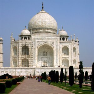
Original Taj Image

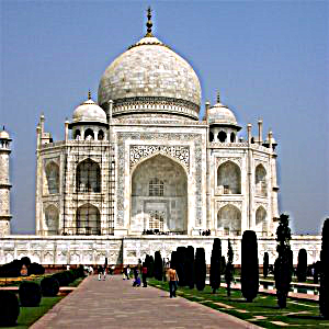
Sharpened Taj Image

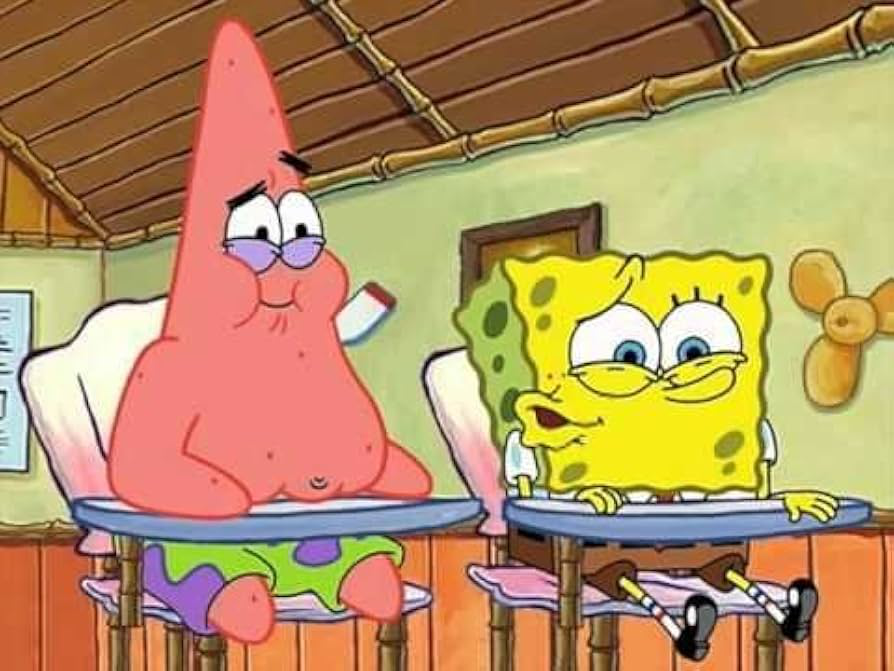
Original Spongebob Image

Blurred Spongebob Image

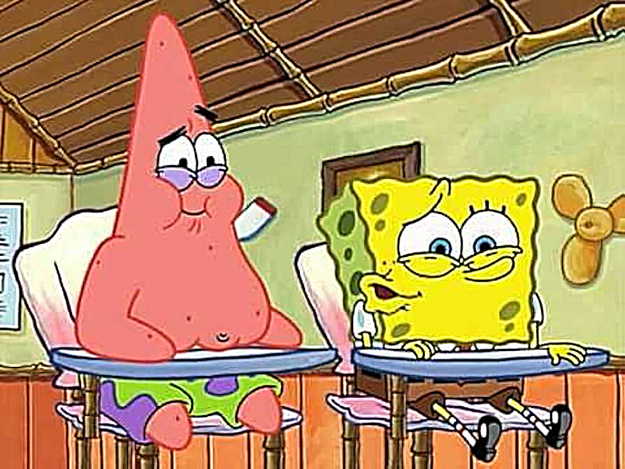
Sharpened Spongebob Image

2.2: Hybrid Images

By combining the high-frequency content of one image and the low-frequency content of another, we create a hybrid image that changes in interpretation based on viewing distance. Below, we showcase three examples of hybrid images: Derek and the Cat, Batman and Joker, and Sri and the Dog.

Derek and the Cat

In this example, we blend the high-frequency content of Derek's face with the low-frequency content of a cat's face. You may need to zoom in to see the whiskers popping out in the hybrid image.

Fourier Analysis of Original Images - Derek and Cat

The Fourier transform of the original images helps visualize the frequency content of each image before any filtering or blending. Below are the Fourier transforms of the original Derek and Cat images.

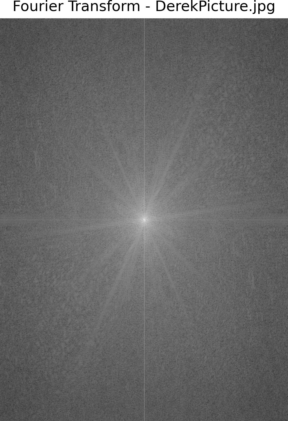
Fourier Transform of Original Derek

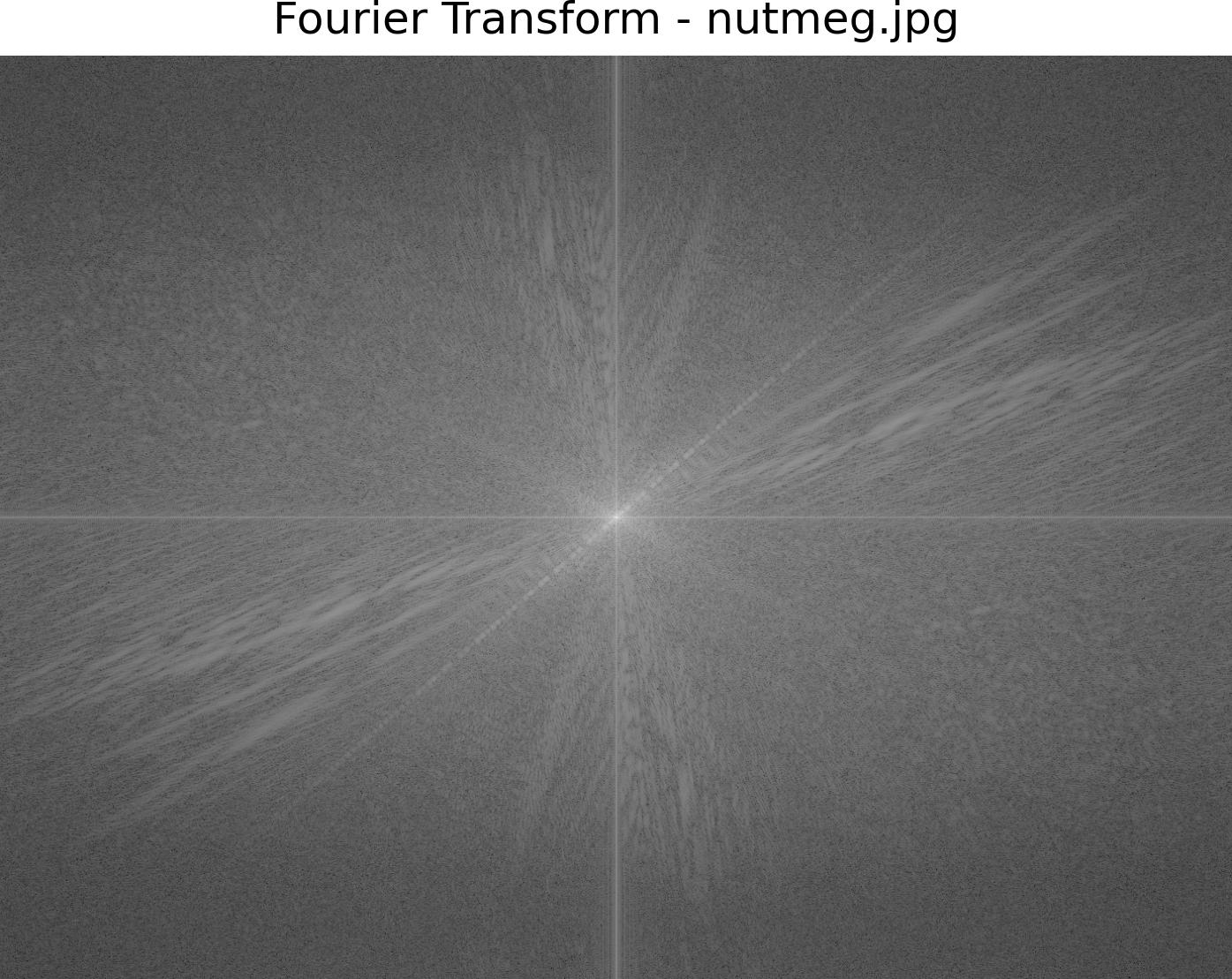
Fourier Transform of Original Cat

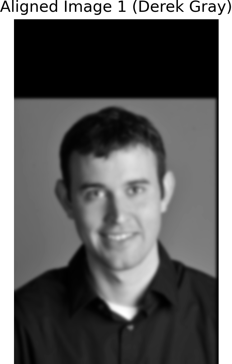
Low-Pass Image of Derek

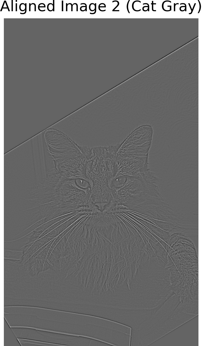
High-Pass Image of Cat

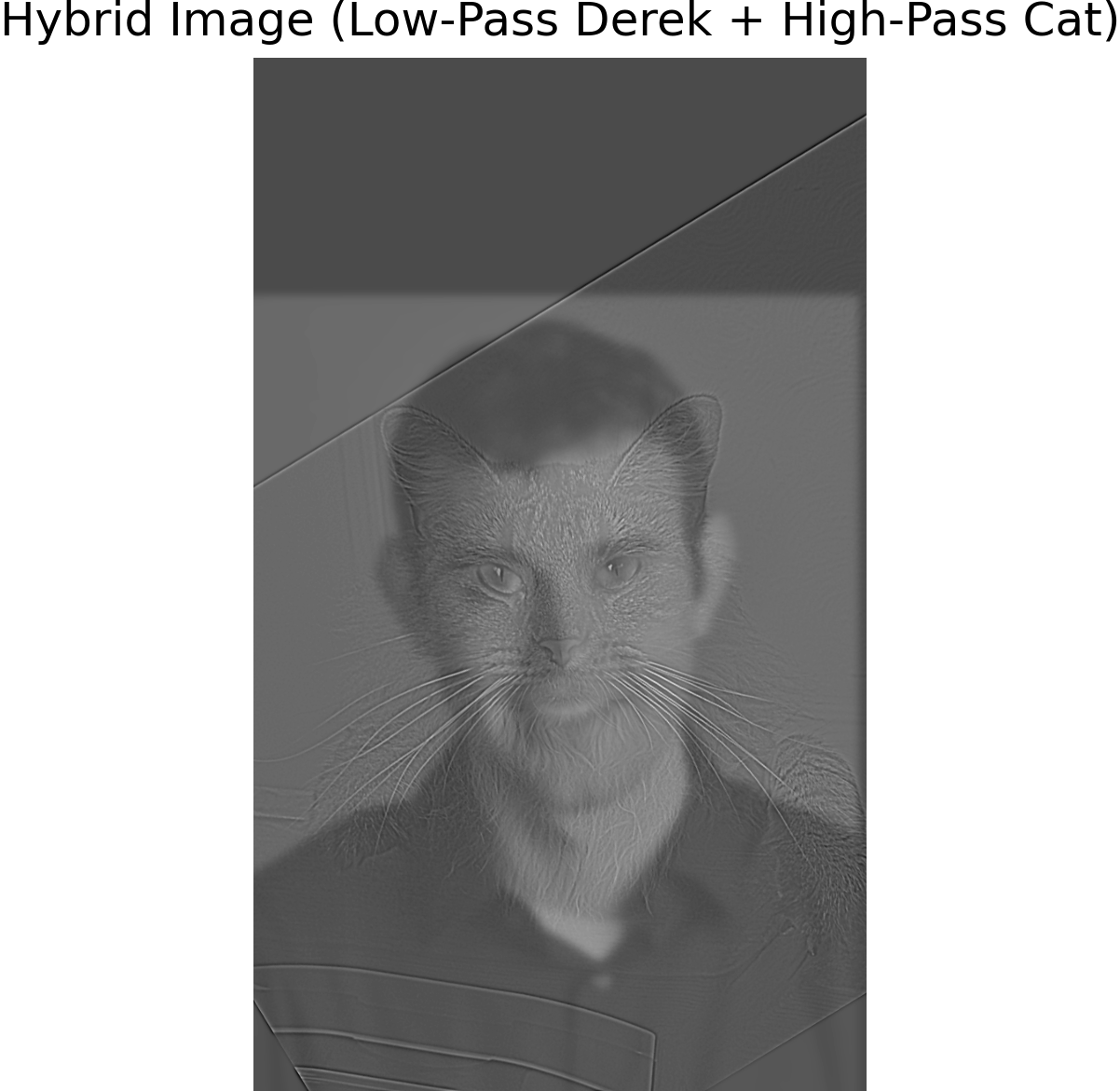
Hybrid Image of Derek and Cat

Fourier Analysis - Derek and Cat

Below, we display the log magnitude of the Fourier transform for the low-pass and high-pass filtered images, as well as the hybrid image. The Fourier transform helps visualize the frequency content of each image, highlighting the distinct high and low frequencies.

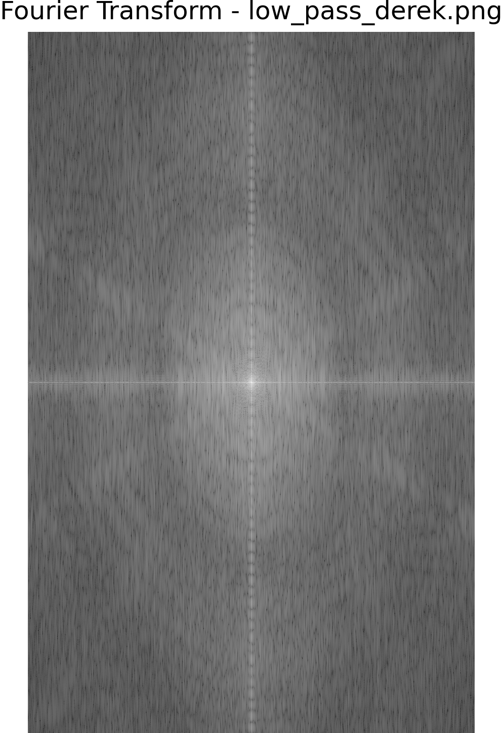
Fourier Transform of Low-Pass Derek

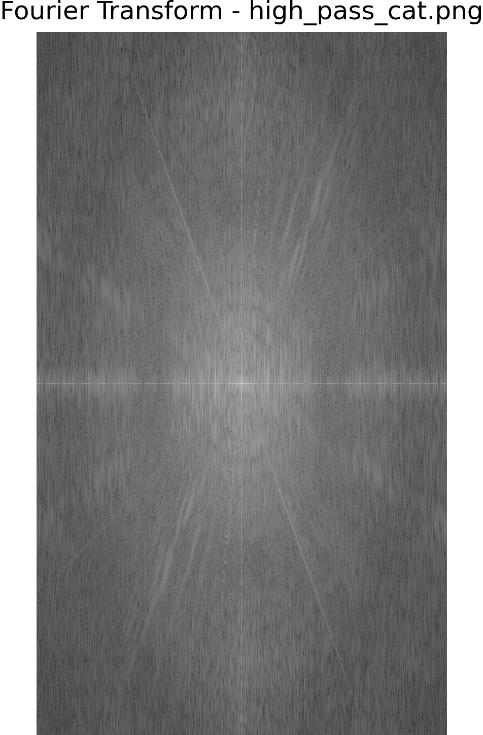
Fourier Transform of High-Pass Cat

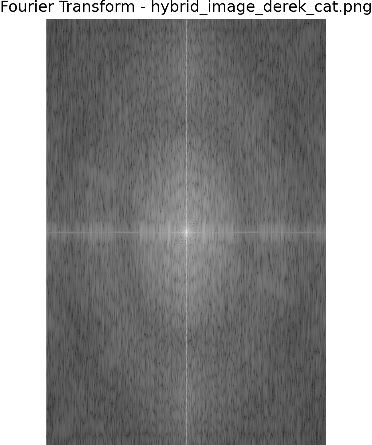
Fourier Transform of Hybrid Derek and Cat

Batman and Joker

In this example, we blend the high-frequency content of Joker's face with the low-frequency content of Batman's face. Up close, you can see the details of Joker's face, while from a distance, the blended image takes on the appearance of Batman.

Fourier Analysis of Original Images - Batman and Joker

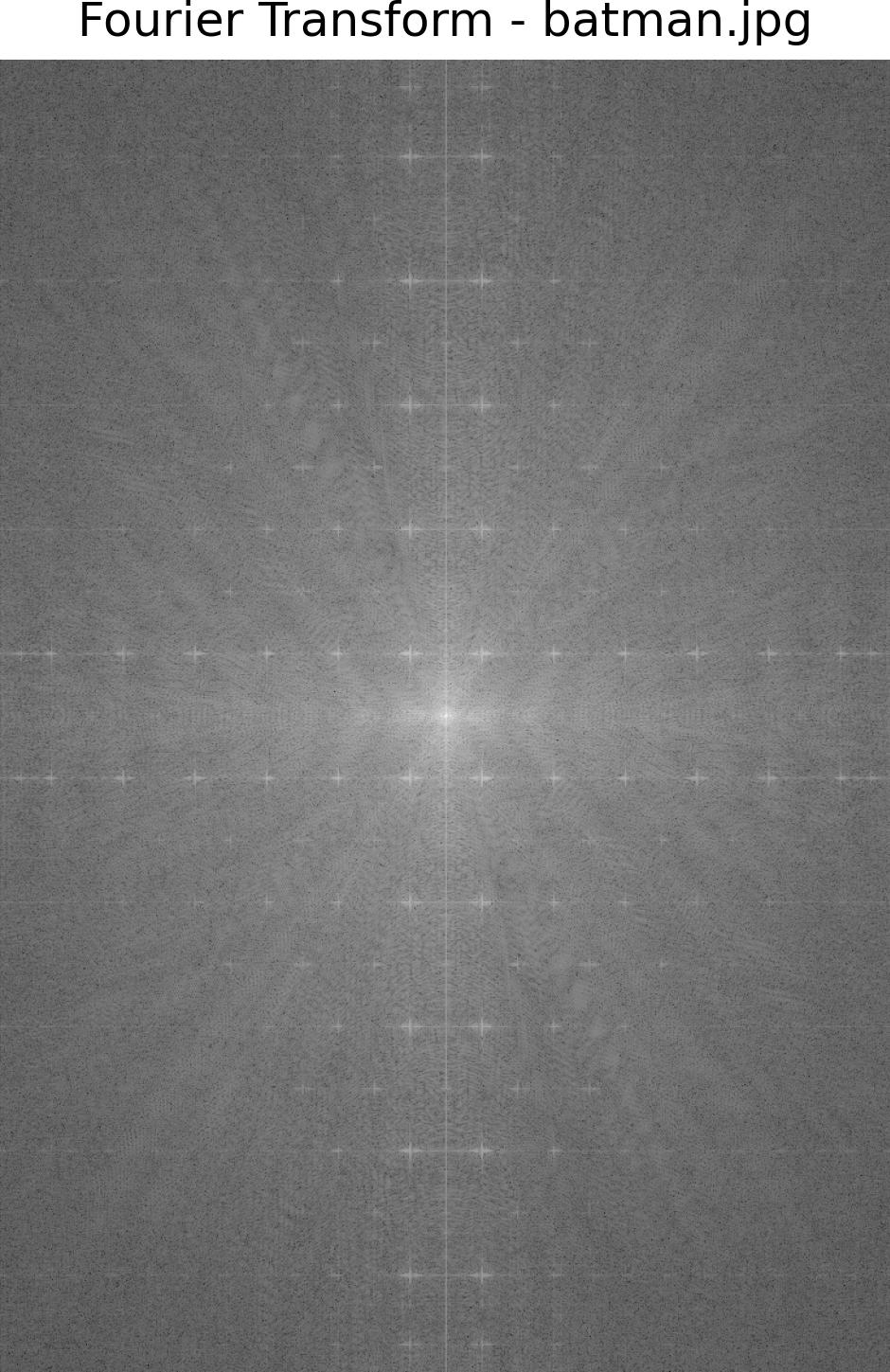
Fourier Transform of Original Batman

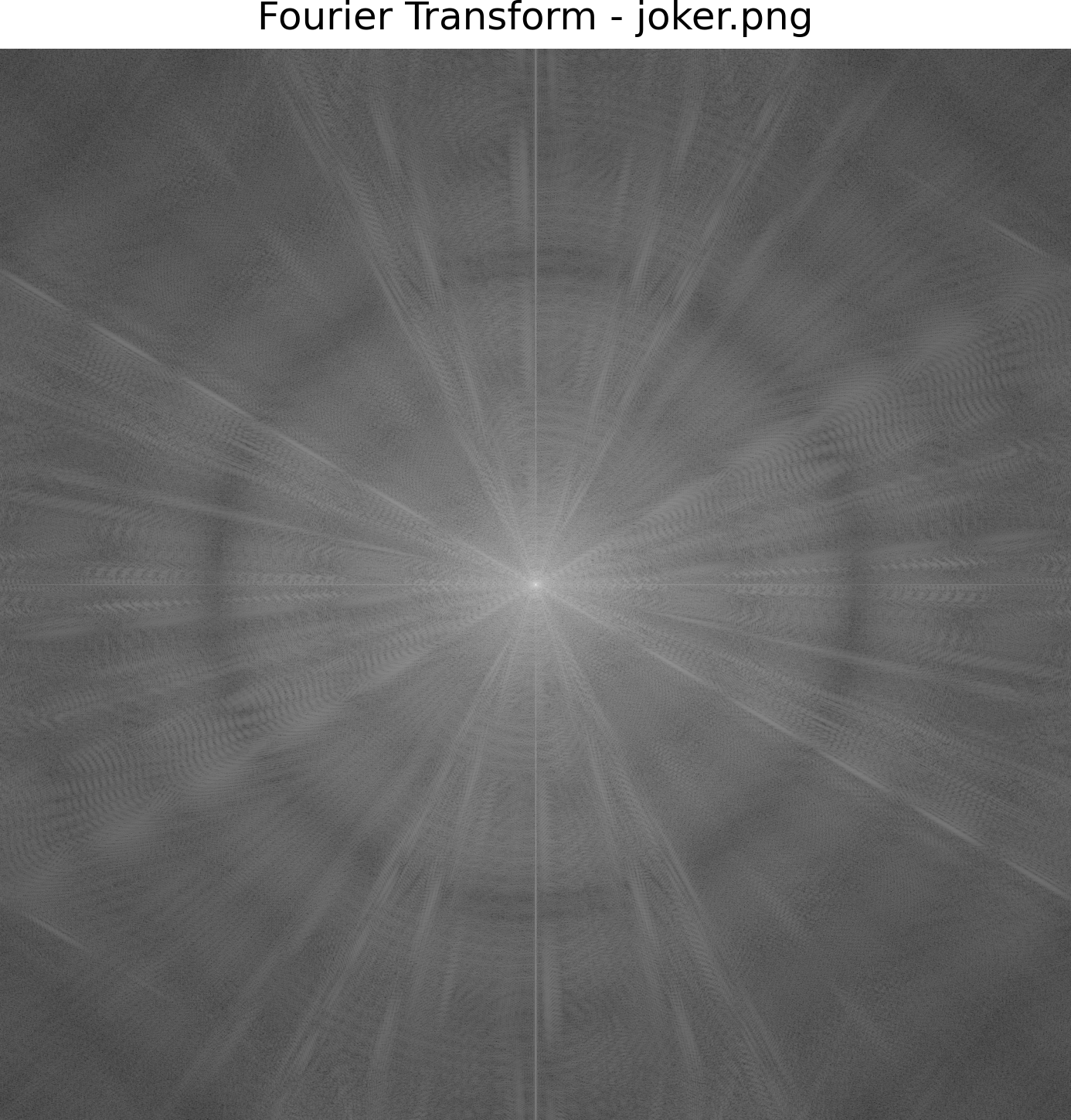
Fourier Transform of Original Joker

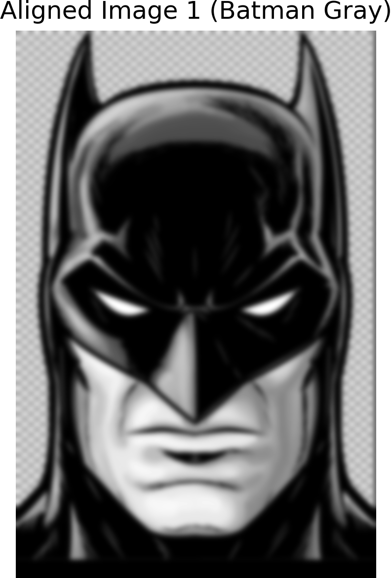
Low-Pass Image of Batman

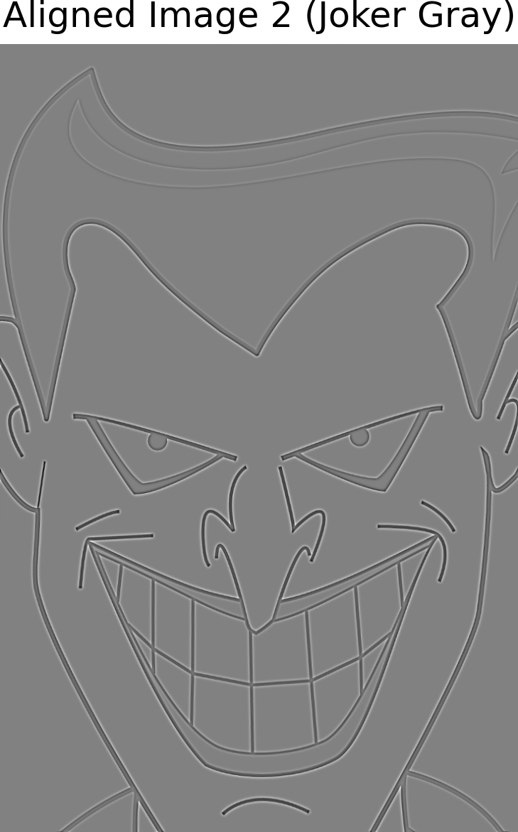
High-Pass Image of Joker

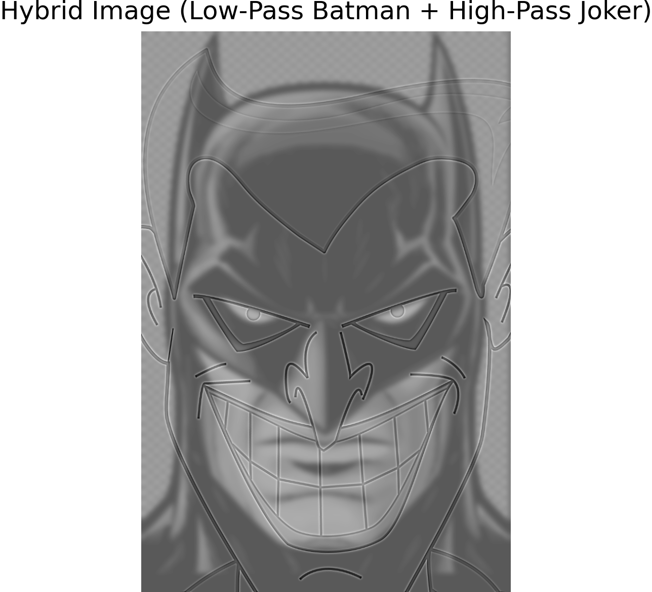
Hybrid Image of Batman and Joker

Fourier Analysis - Batman and Joker

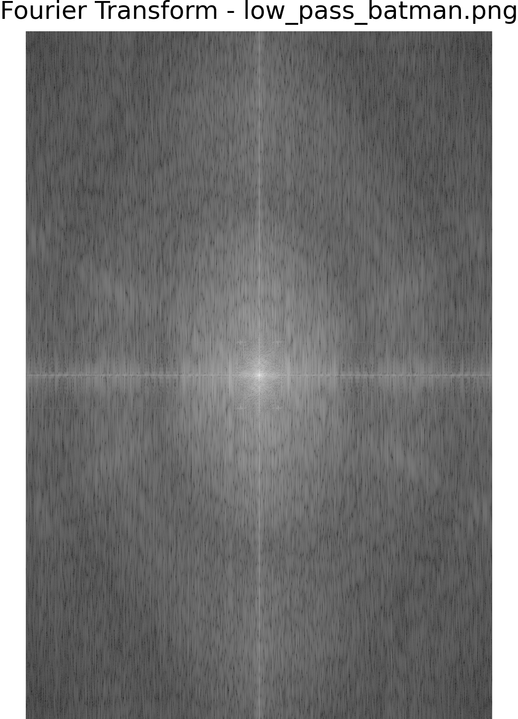
Fourier Transform of Low-Pass Batman

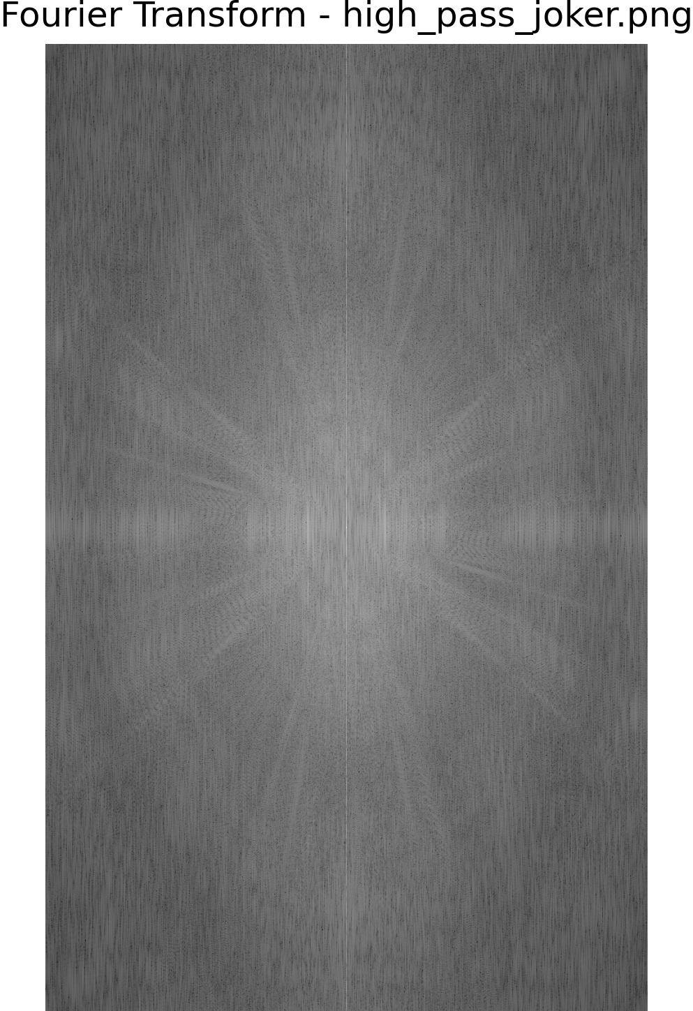
Fourier Transform of High-Pass Joker

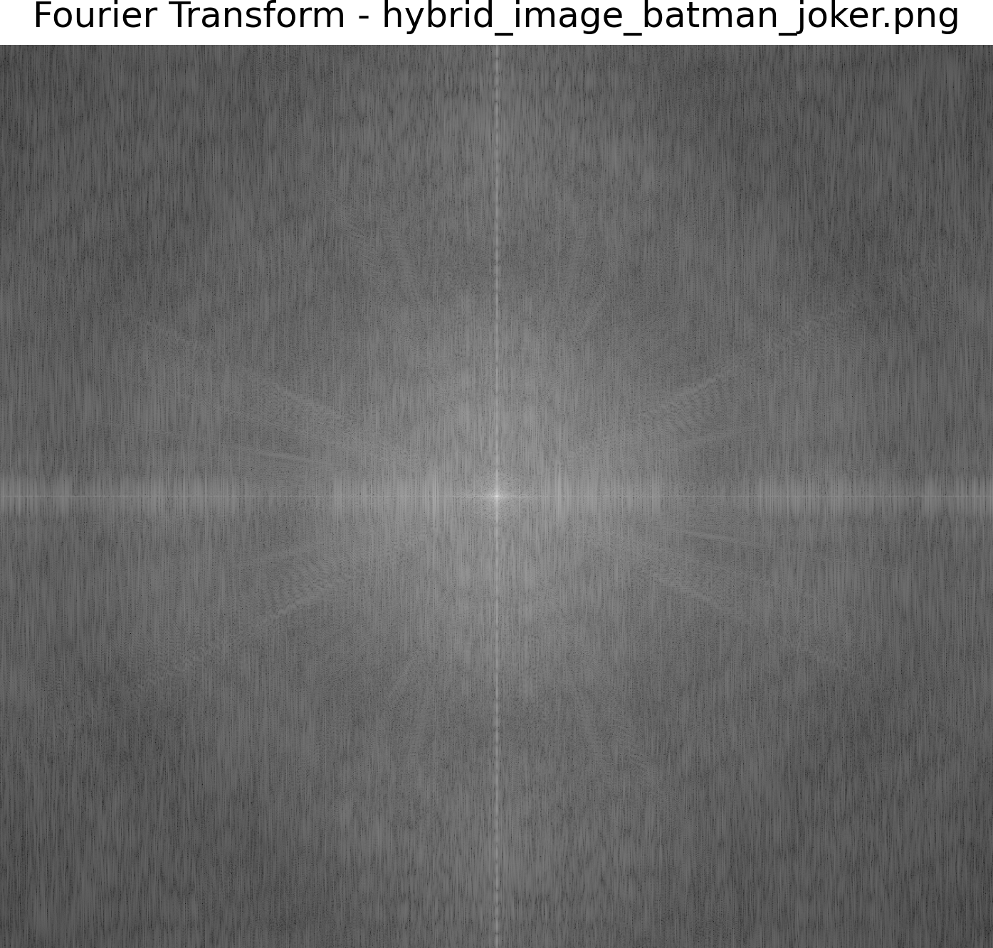
Fourier Transform of Hybrid Batman and Joker

Sri and the Dog (Failed Example)

For this hybrid image, we attempted to blend the high-frequency content of Sri's face with the low-frequency content of a dog's face using a high pass and low pass filter. The goal was to create a seamless transition between the two images. However, due to poor alignment and contrasting features, the resulting image did not blend well. Up close, the details of Sri's face are apparent, but the overall hybrid image appears distorted and fails to capture the desired effect. The dog essentially got nullified so the merged image does not look right.

Fourier Analysis of Original Images - Sri and Dog

The Fourier transform of the original images helps visualize the frequency content of each image before any filtering or blending. Below are the Fourier transforms of the original Sri and Dog images.

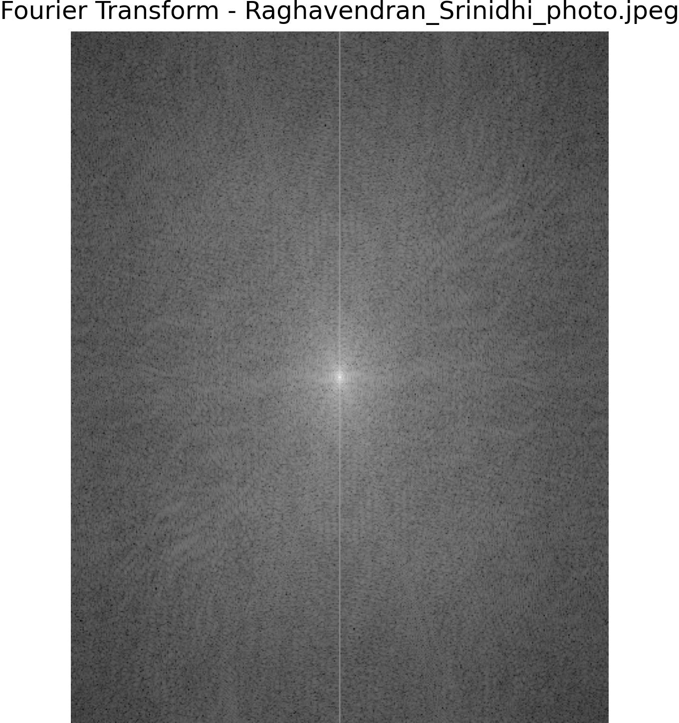
Fourier Transform of Original Sri

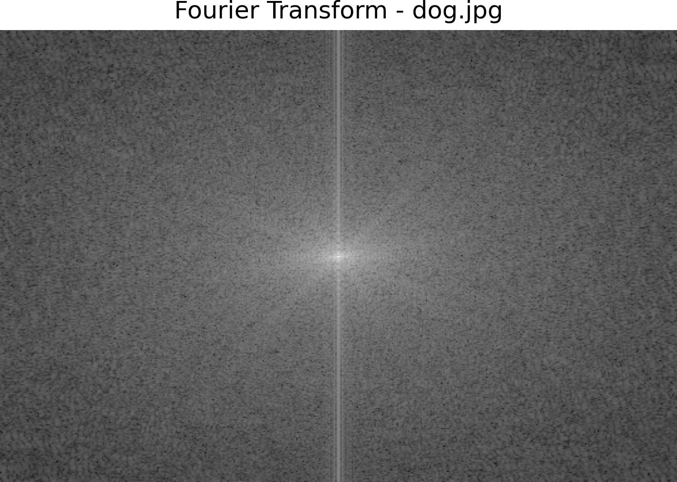
Fourier Transform of Original Dog

Low-Pass Image of Sri

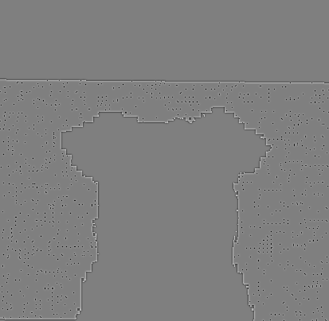
High-Pass Image of Dog

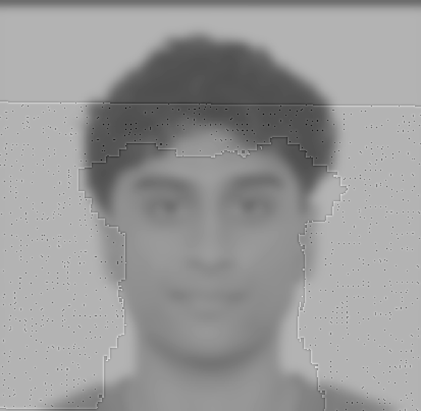
Hybrid Image of Sri and Dog (Failed)

Fourier Analysis - Sri and Dog

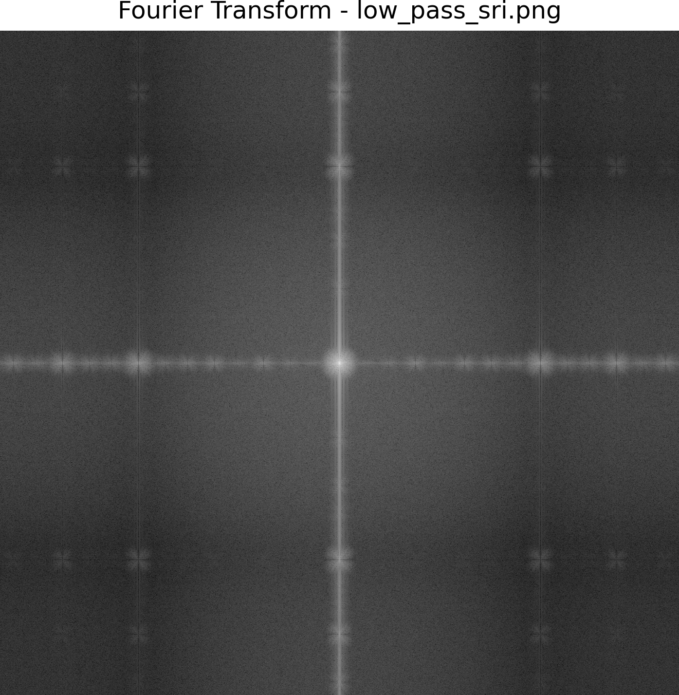
Fourier Transform of Low-Pass Sri

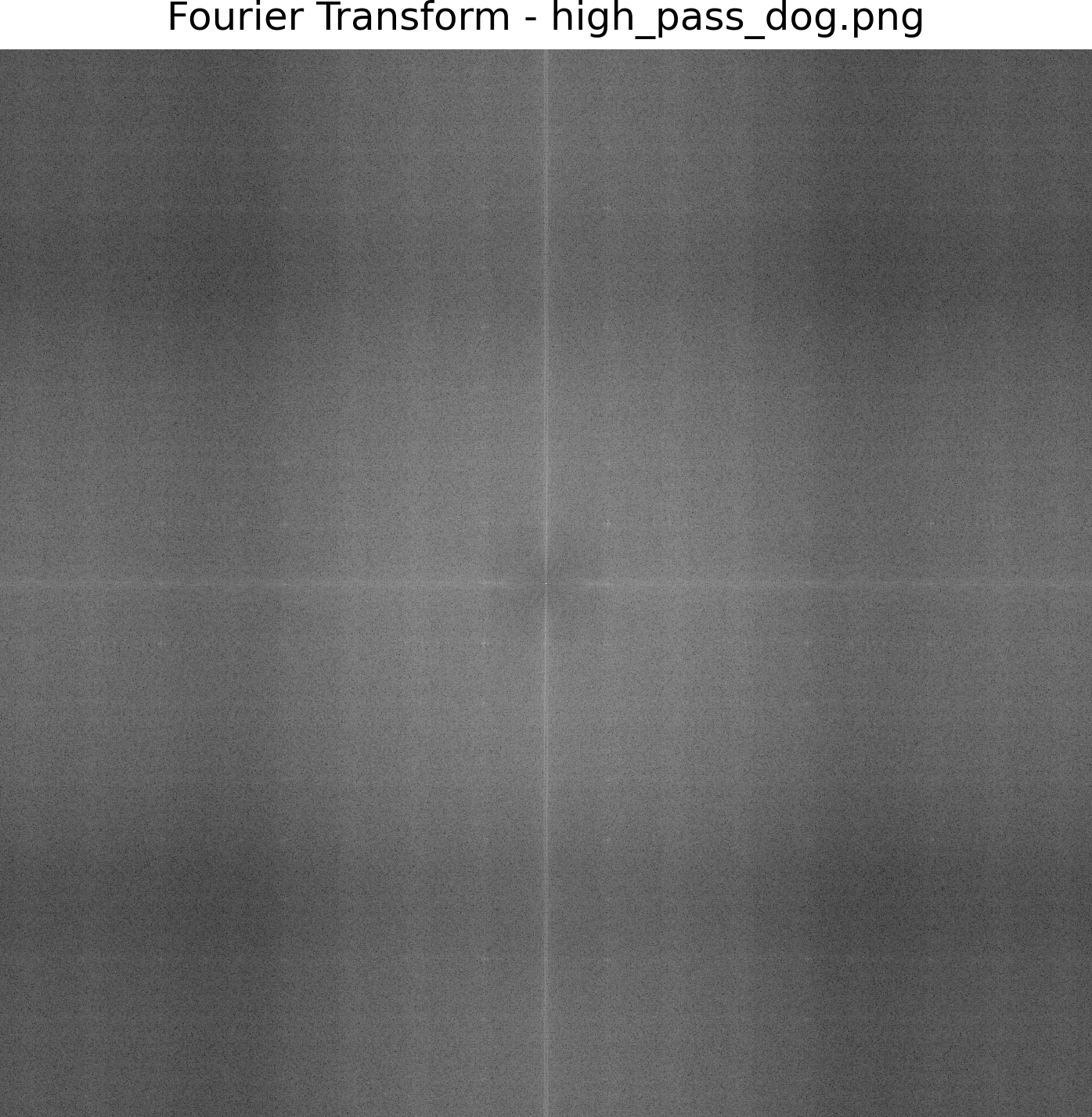
Fourier Transform of High-Pass Dog

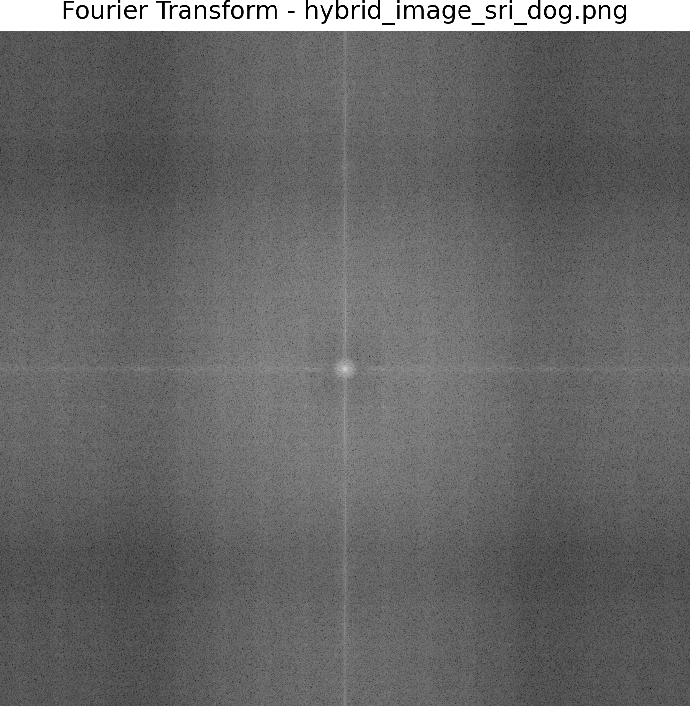
Fourier Transform of Hybrid Sri and Dog

2.3: Gaussian and Laplacian Stacks

We created Gaussian and Laplacian stacks at different levels (0, 2, and 4) for both the apple and orange images, which allowed us to capture high, medium, and low-frequency details without downsampling. Below, we display a visualization of the Laplacian blending process for these levels.

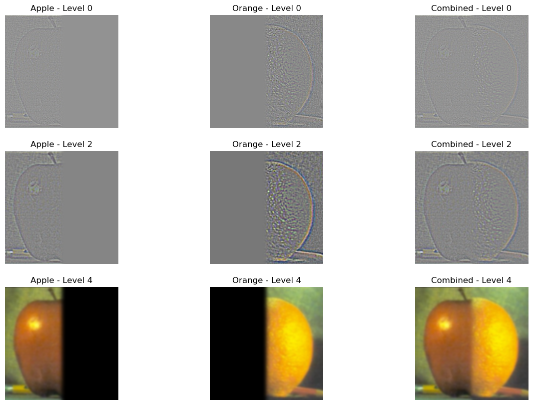
Laplacian Blending at Levels 0, 2, and 4

Part 2.4: Multiresolution Blending

By implementing Gaussian and Laplacian stacks, we blend two images seamlessly with smooth transitions, as described in Burt and Adelson's paper. For this blending experiment, we used an image of a goblin and a photo of Sri. An intermediate step involved aligning the two images since their original sizes were different. We used an alignment function from section 2.2 to adjust the images to the same size and orientation before blending.

We used an irregular mask in the shape of a circle to blend the two images. The circular mask ensures a smooth transition between the goblin and Sri, where the blending happens predominantly in the center of the image. The edges of the mask were blurred to achieve a seamless blend across different levels of the Gaussian and Laplacian stacks.

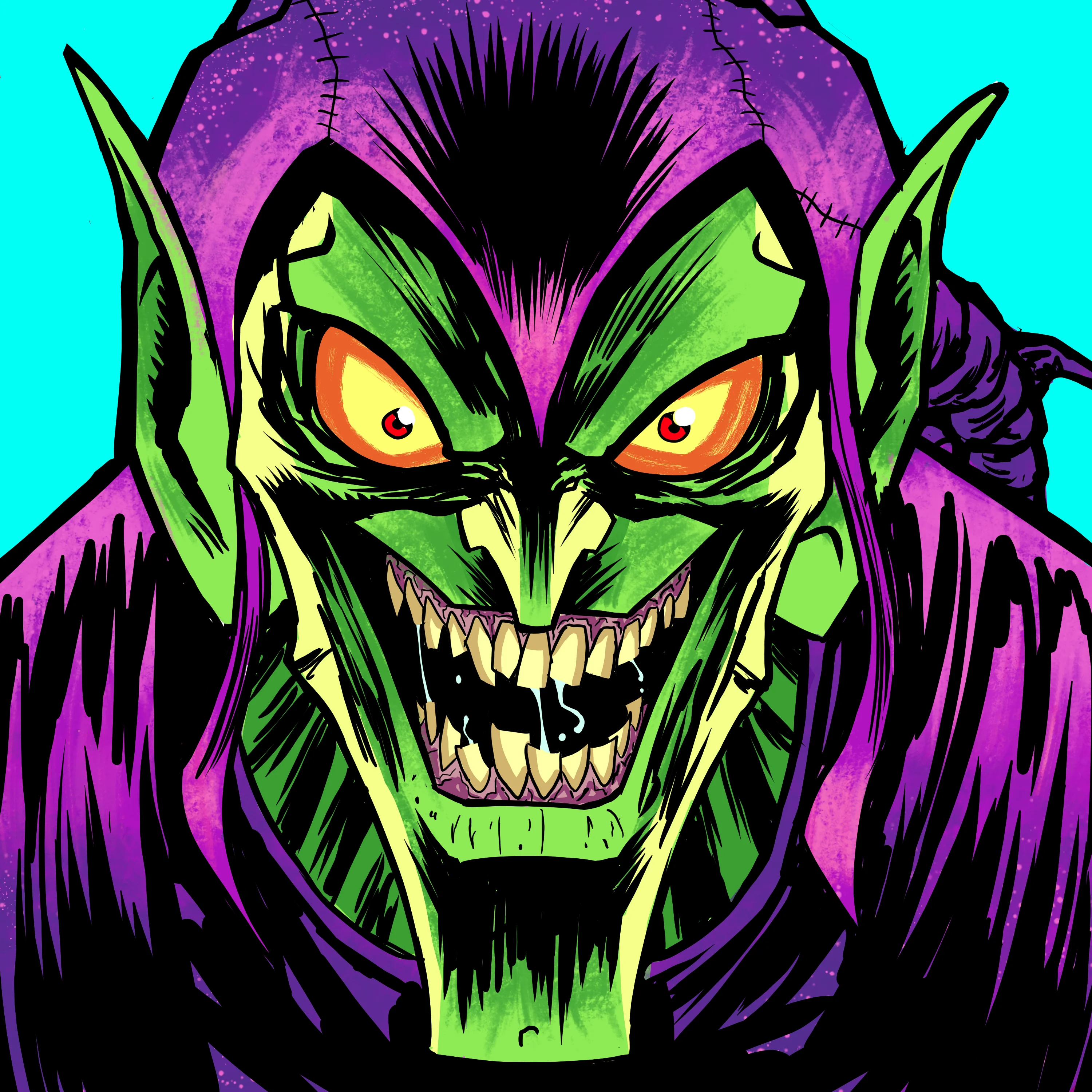
Original Goblin Image

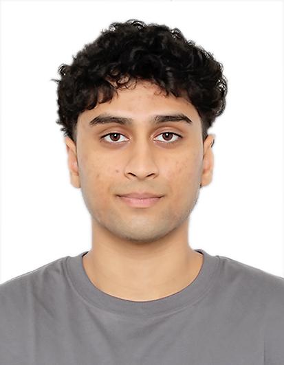
Original Sri Image

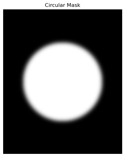
Circular Mask

Laplacian Blending at Different Levels

Below is the Laplacian blended image at different levels (0, 2, and 4) using the circular mask. The images of the goblin and Sri are blended smoothly at each level using the Gaussian and Laplacian pyramids, creating a single visualization.

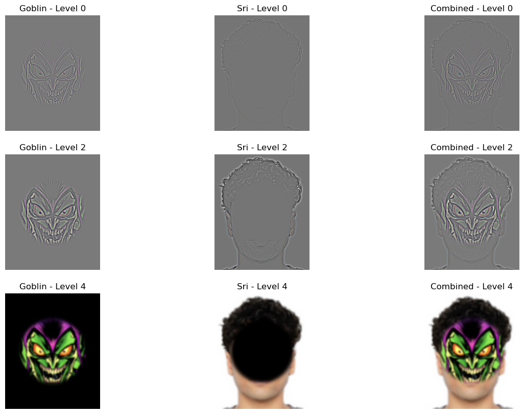
Blending at Levels 0, 2, and 4

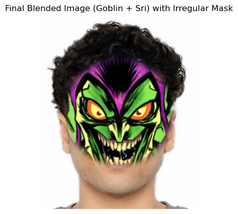
Final Blended Image (Goblin + Sri) with Circular Mask

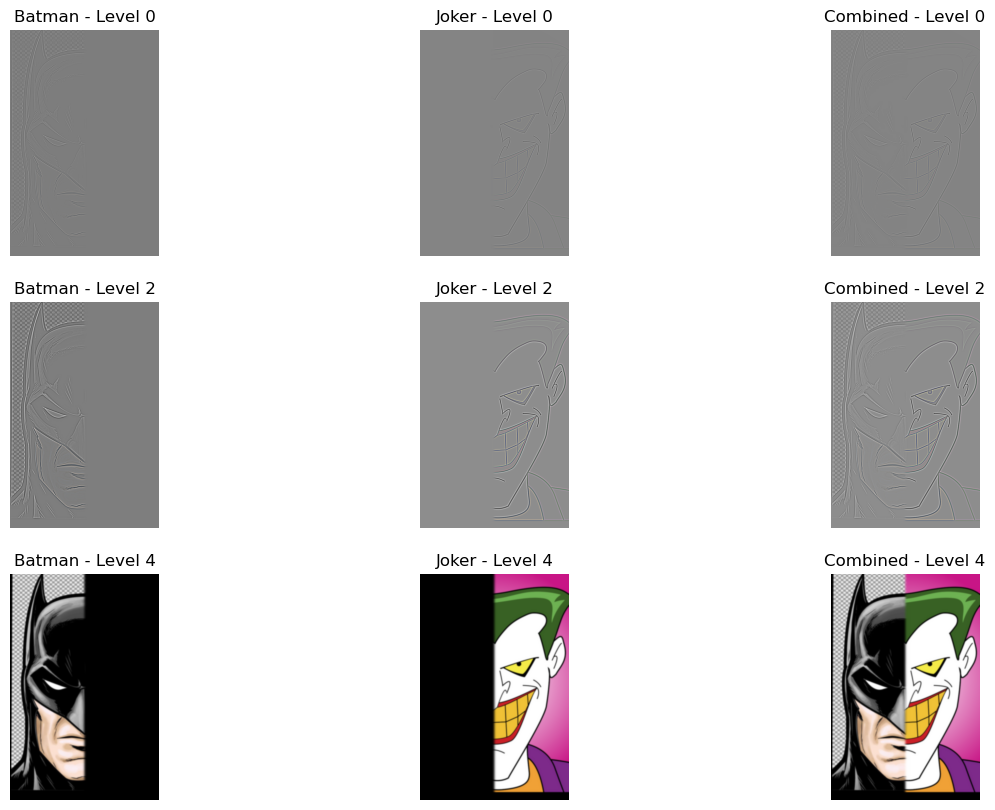
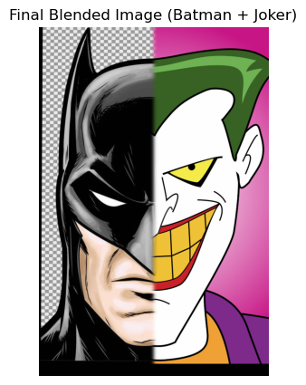
Part 2.4: Multiresolution Blending (Batman + Joker)

In this blending experiment, we combined images of Batman and Joker. Similar to the previous example, an intermediate step involved aligning the two images since they had different sizes and orientations. The alignment function used in section 2.2 was applied to resize and adjust the images before creating Gaussian and Laplacian stacks for multi-resolution blending.

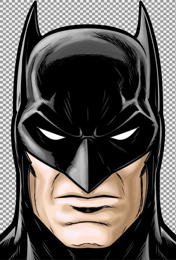
Batman Image

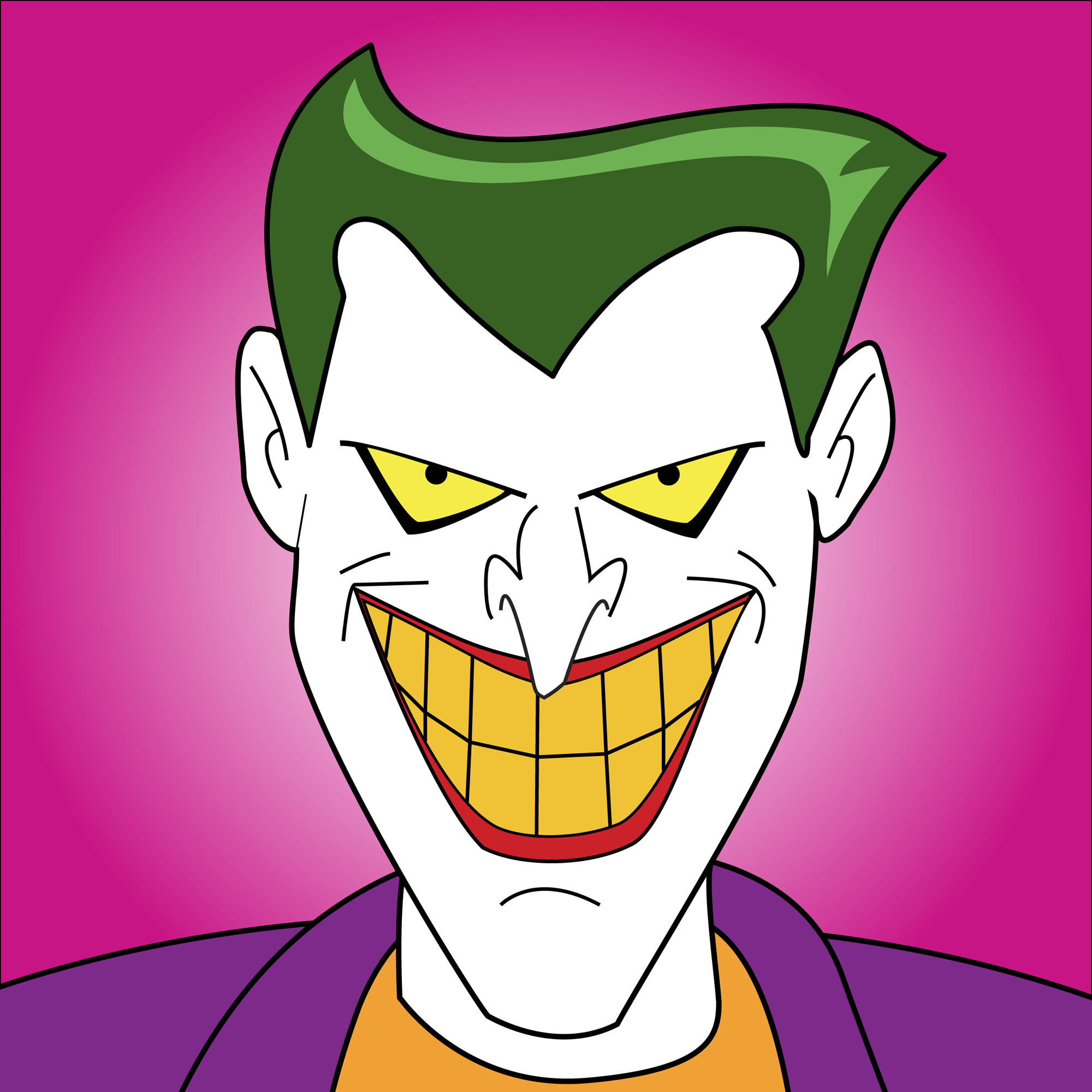
Joker Image

Laplacian Blended Levels

Final Blended Image (Batman + Joker)