Image Warping and Mosaicing: CS180 Project 4

Overview - Part A

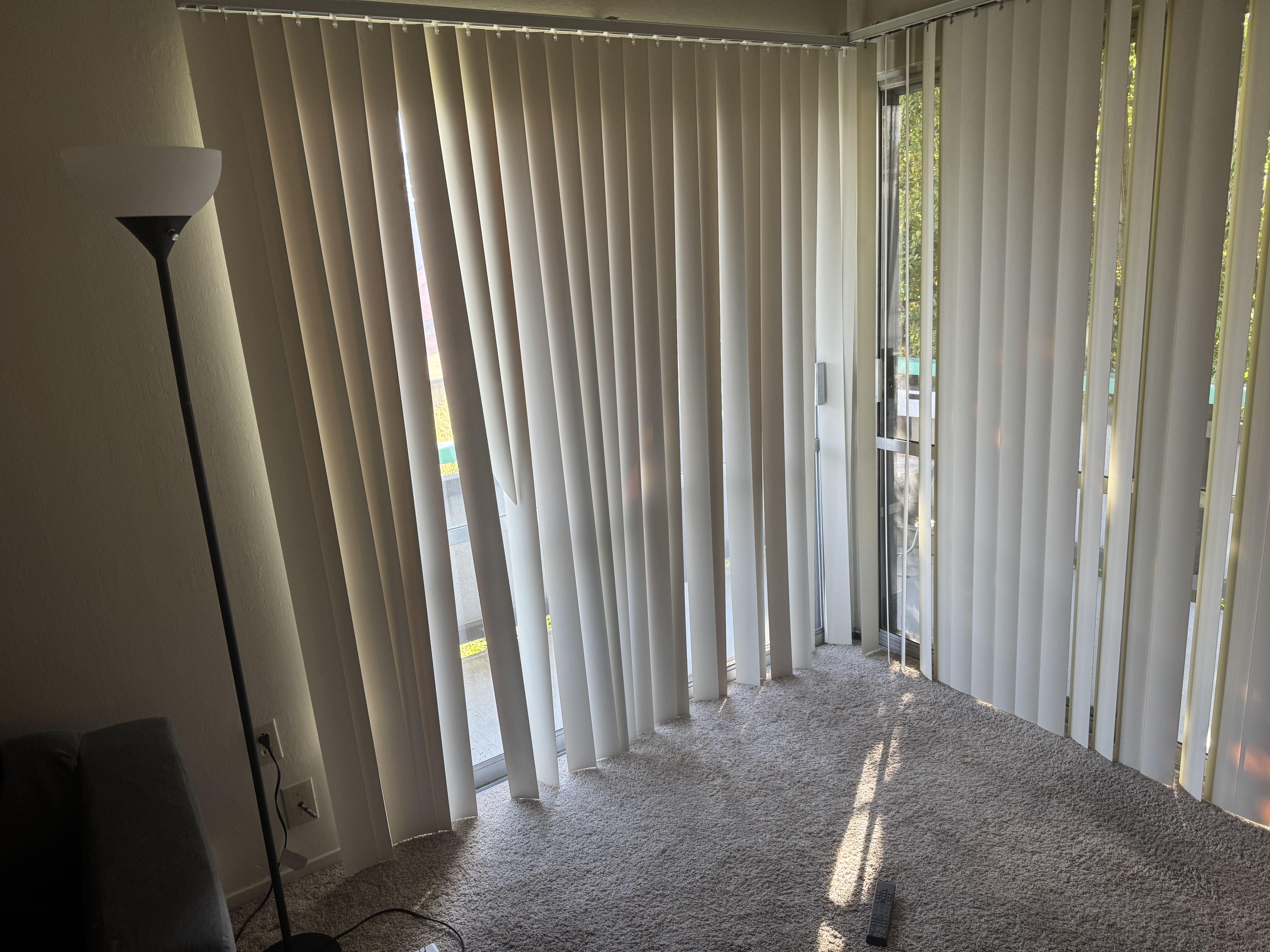
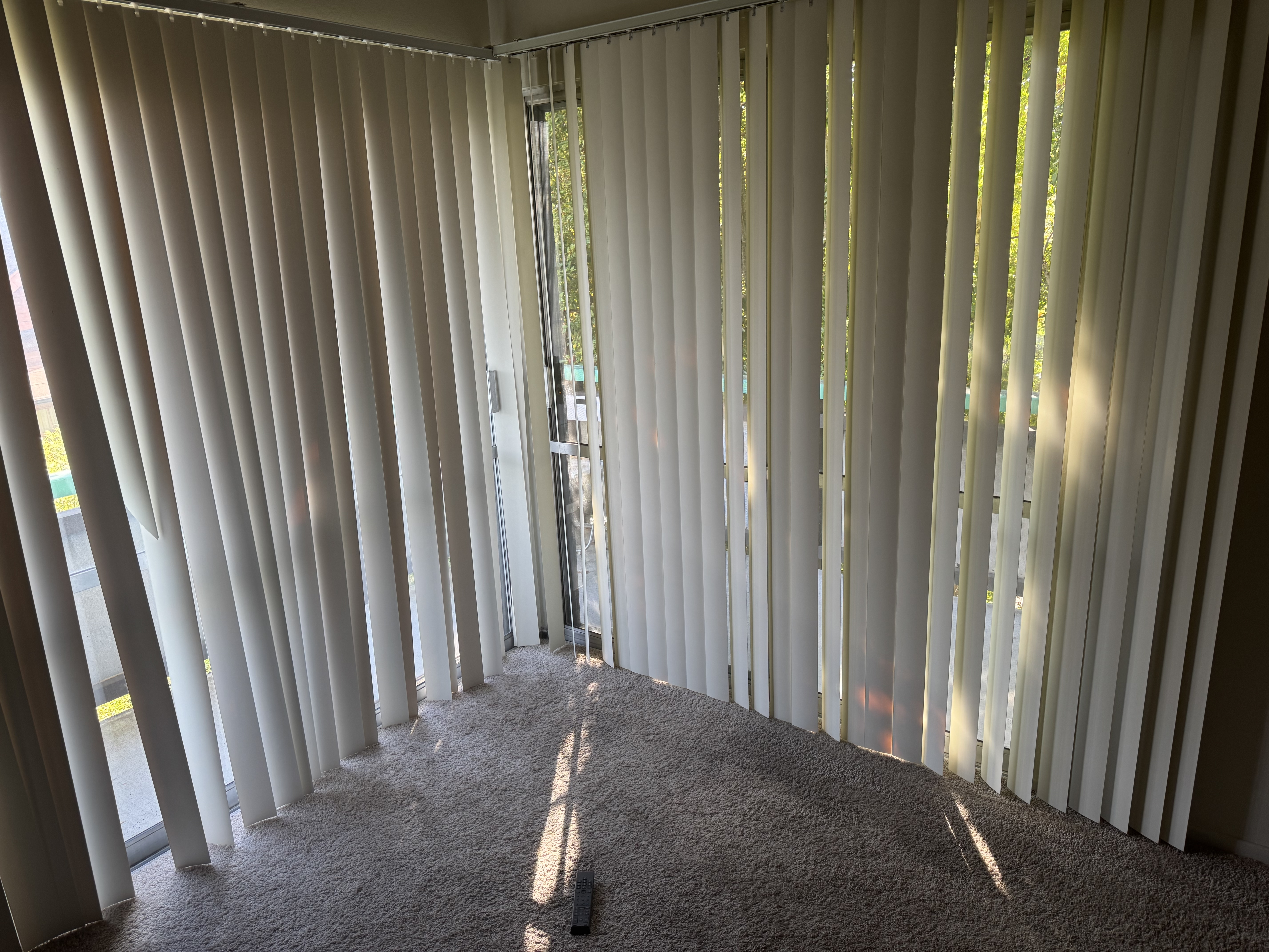
In this project, I explored various image warping techniques to create mosaics using multiple photographs. The project involved key steps: shooting images, recovering homographies, warping images, and blending them into mosaics. Below, I present the original images for three different scenes: the library, a tile area, and a window.

Part 1: Shoot the Pictures

For each mosaic (library, tile, and window), I shot multiple pictures ensuring significant overlap between the images. This overlap was critical for accurately aligning the images later during homography recovery. I used a fixed center of projection and rotated the camera slightly to capture different views of each scene.

Original Images Used

Library Images

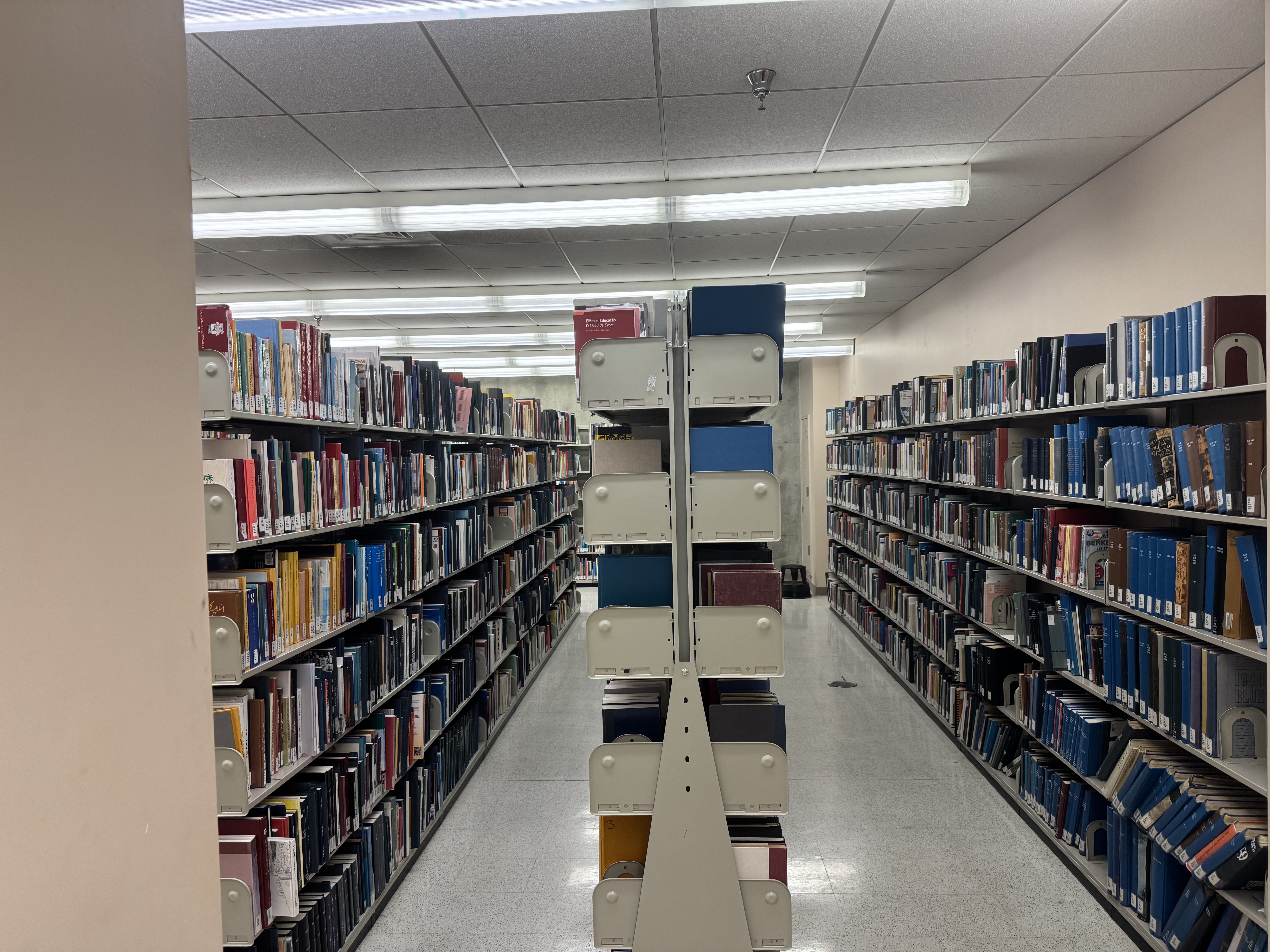
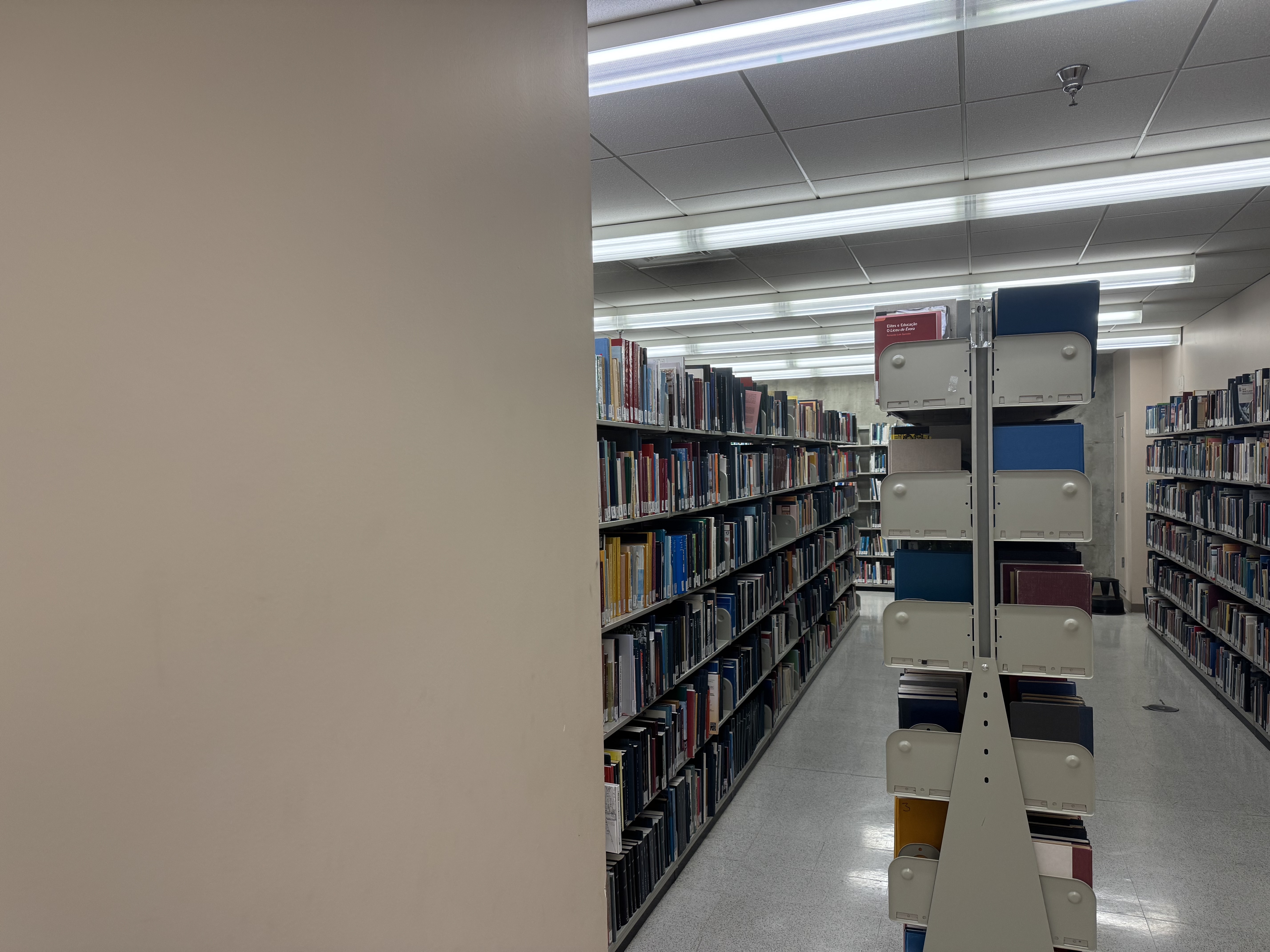
Tile Area Images

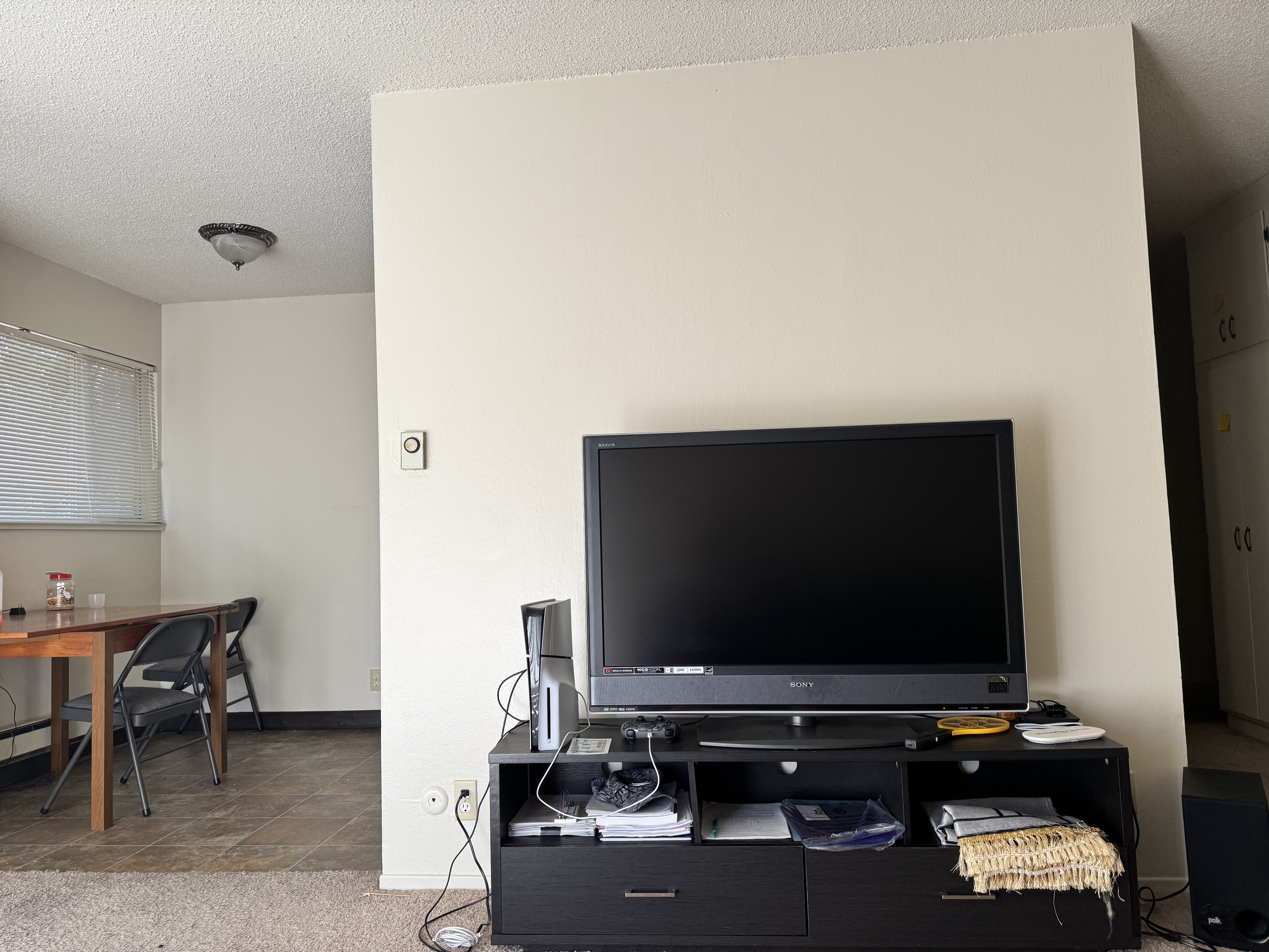
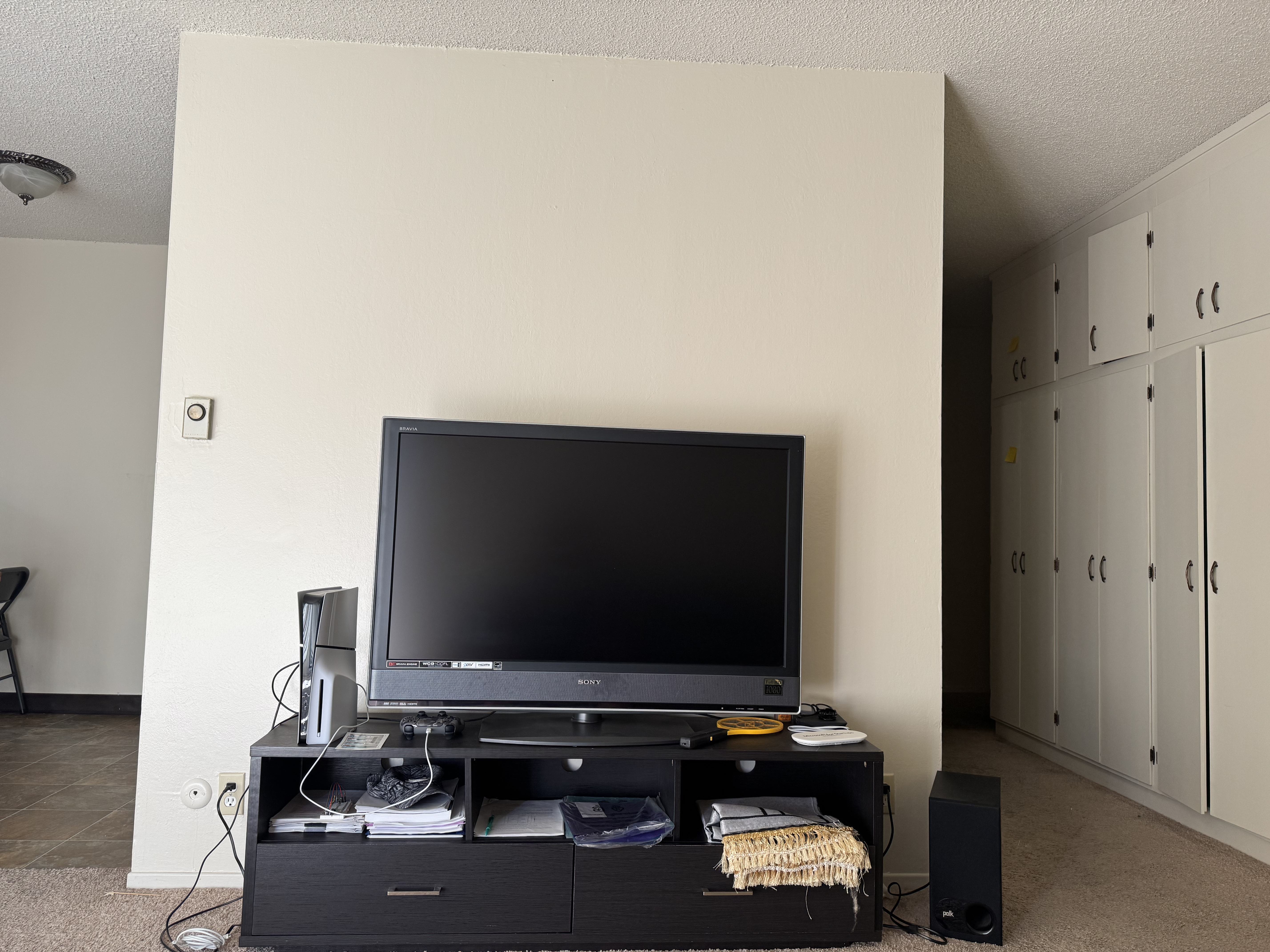
Window Images

Part 2: Recover Homographies

To align the images for each mosaic, I computed the homographies between pairs of images. A homography is a transformation between two planes that preserves straight lines. To recover the homography matrix, I selected several corresponding points from each image and used a least-squares method to solve for the 3x3 homography matrix.

Library Mosaic - Point Correspondences

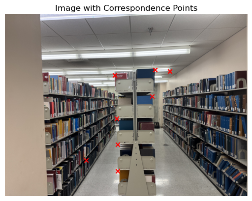
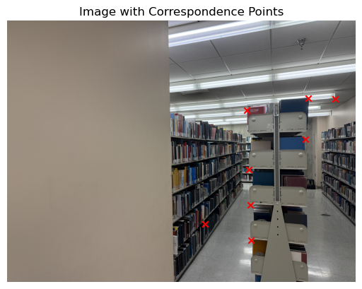
Point Correspondences for the Library Mosaic

Tile Mosaic - Point Correspondences

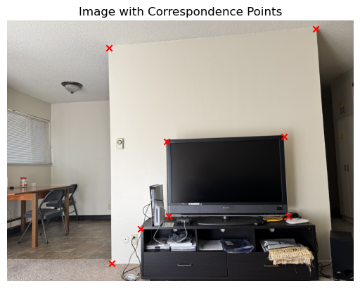
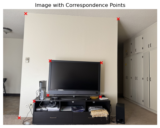
Point Correspondences for the Tile Mosaic

Window Mosaic - Point Correspondences

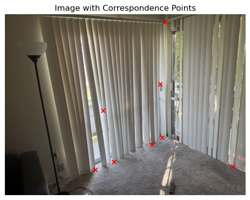
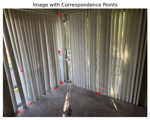
Point Correspondences for the Window Mosaic

Part 3: Warp the Images

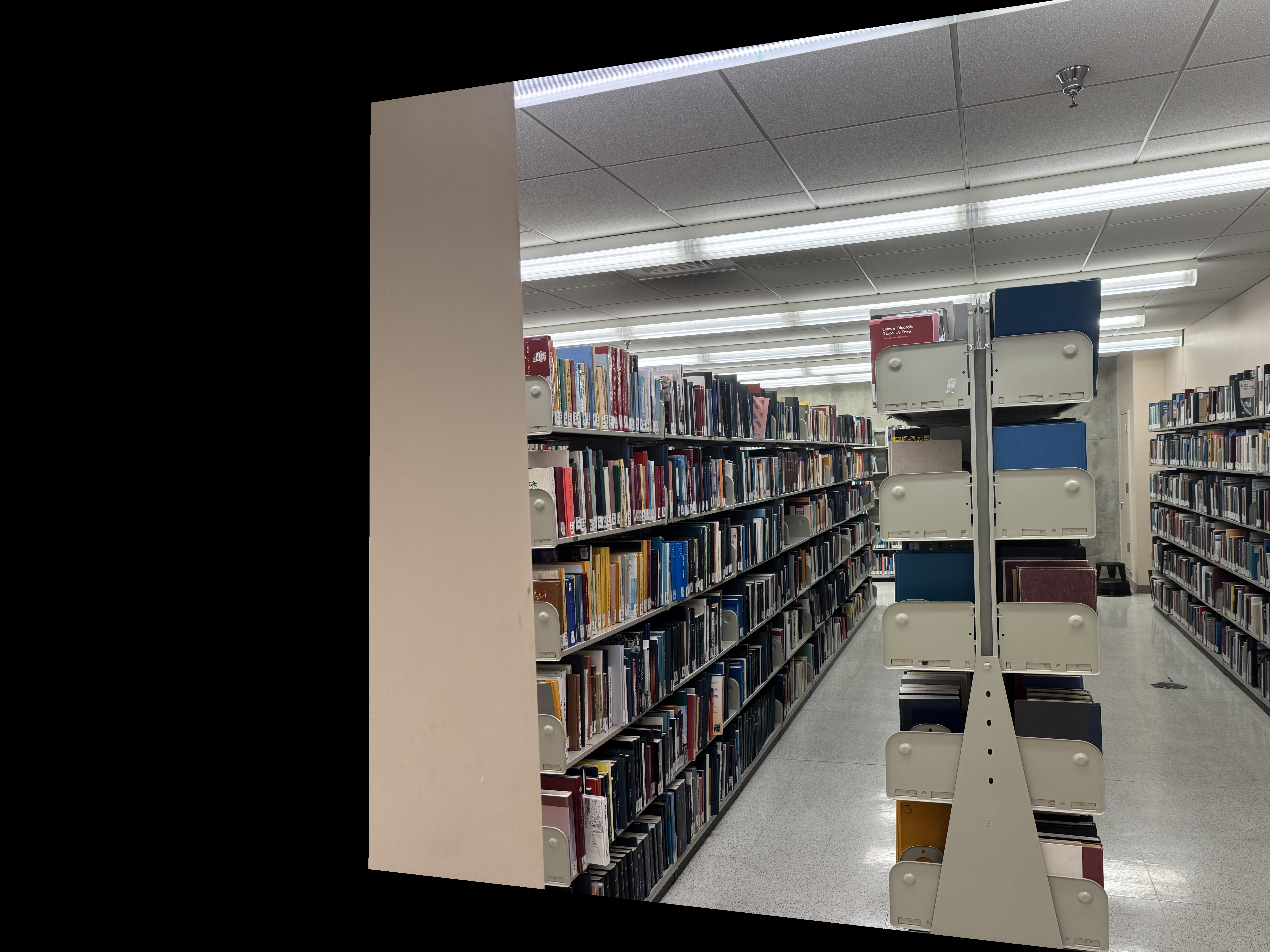
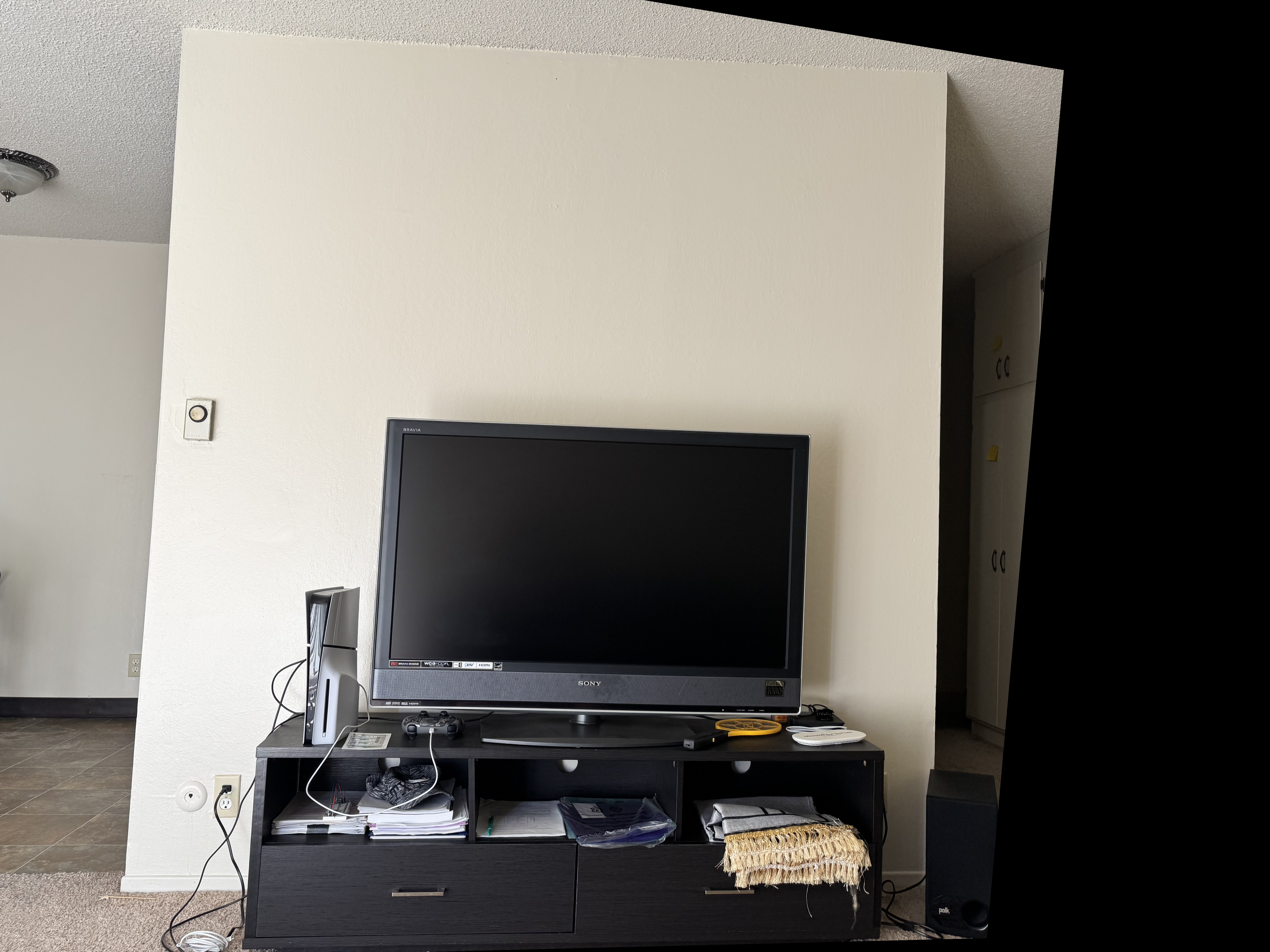
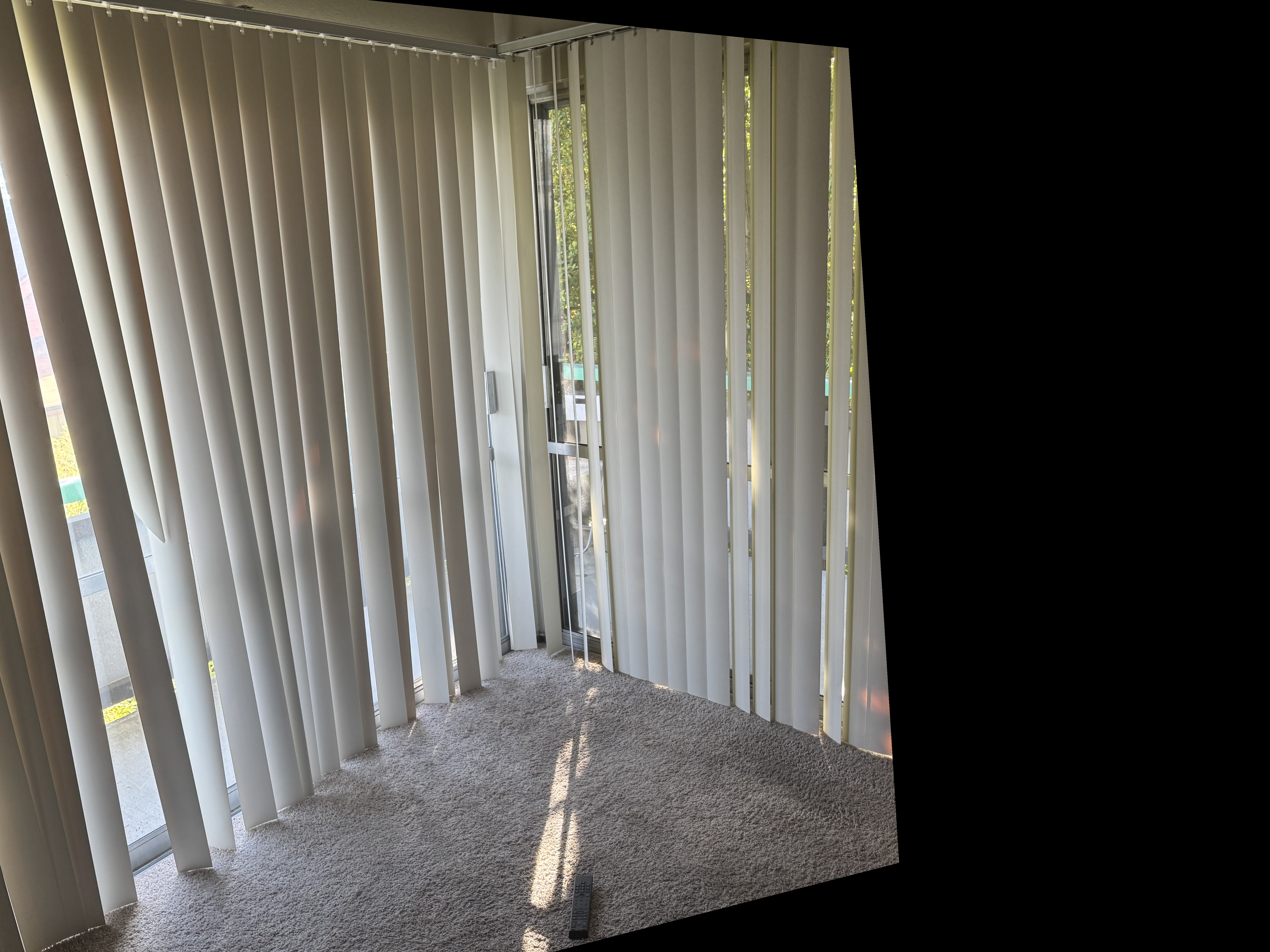
After calculating the homographies, I applied the transformations to warp the images. I implemented a function warpImage(im, H) that takes an image and a homography matrix and outputs the warped image. The transformation aligns the image based on the homography to match the perspective of another image. The resulting warped images for the mosaics are displayed below.

Warped Images

Part 4: Rectification

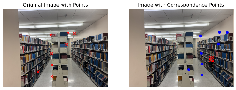
Rectification was used to correct the perspective of objects within the images, making them appear frontal. This was achieved by selecting four corner points of a known rectangle and computing a homography matrix that mapped those points to a rectangular shape. Below are the selected points and the rectified results. Check the right part of the image, which has the four rectified points selected as well as the correspondence points.

Rectification Points

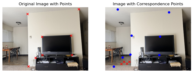
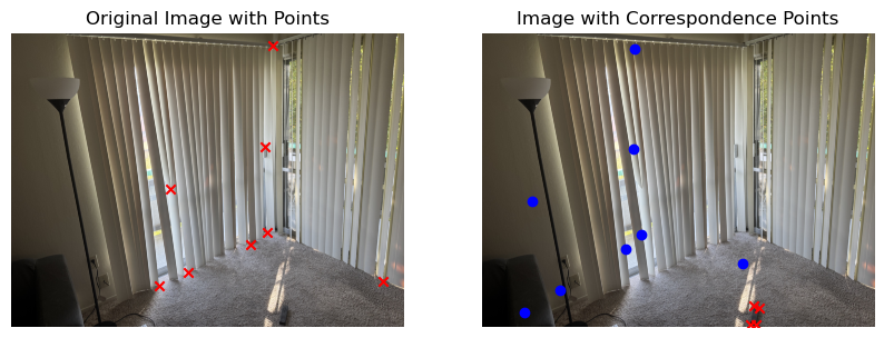
Selected Rectification Points for Each Mosaic

Rectified Images

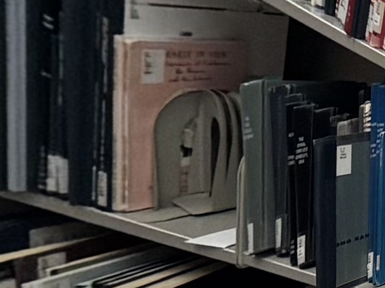
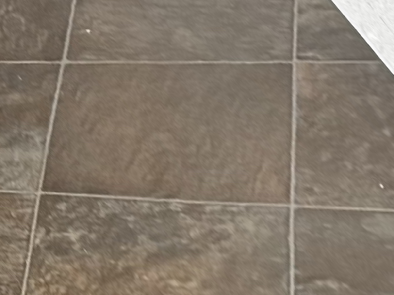
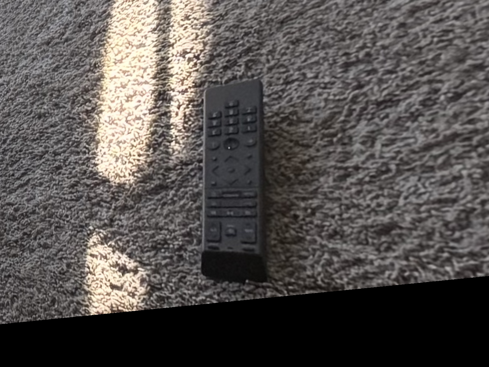
Rectified Results for Each Mosaic

Final Mosaics

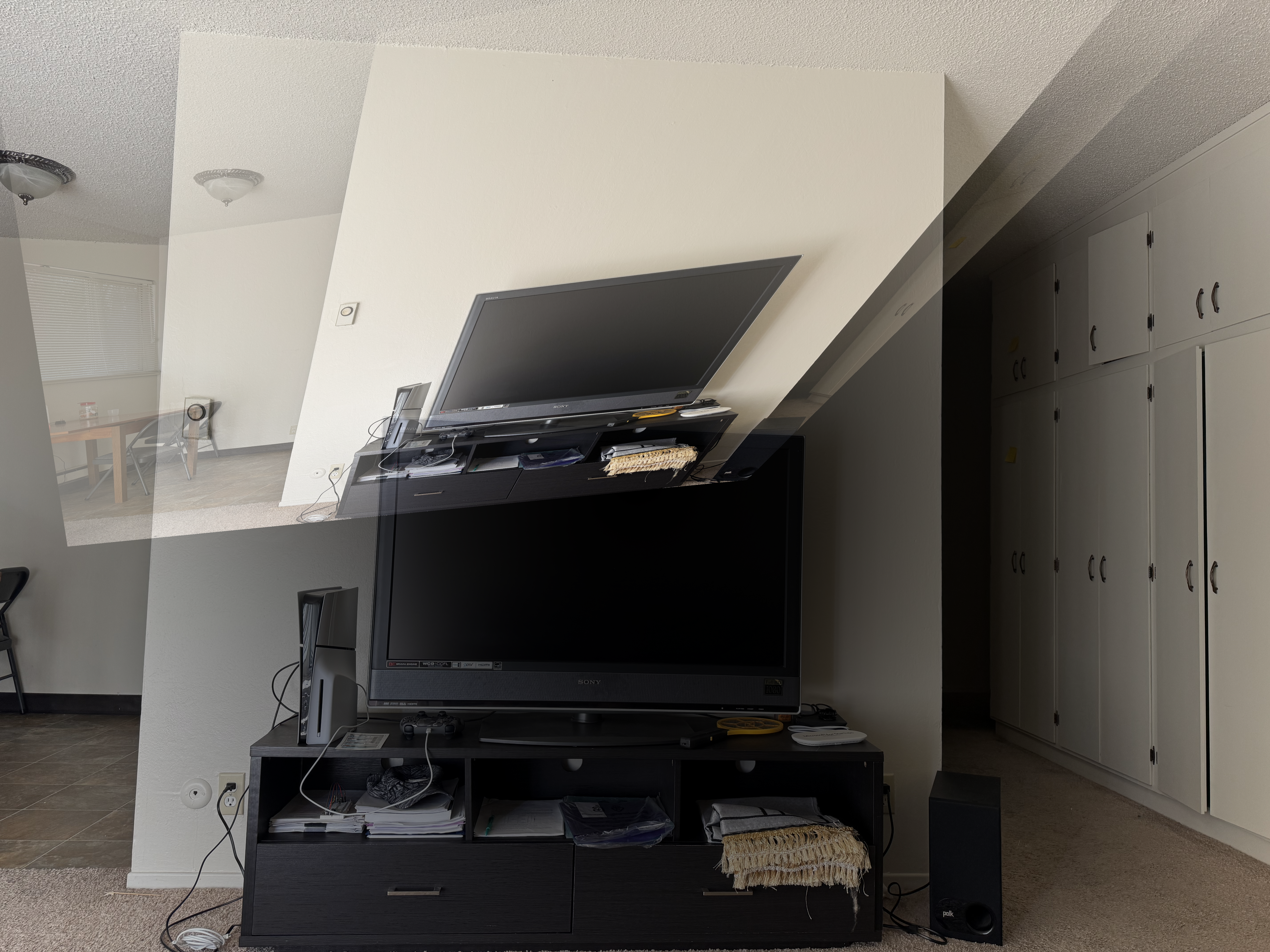
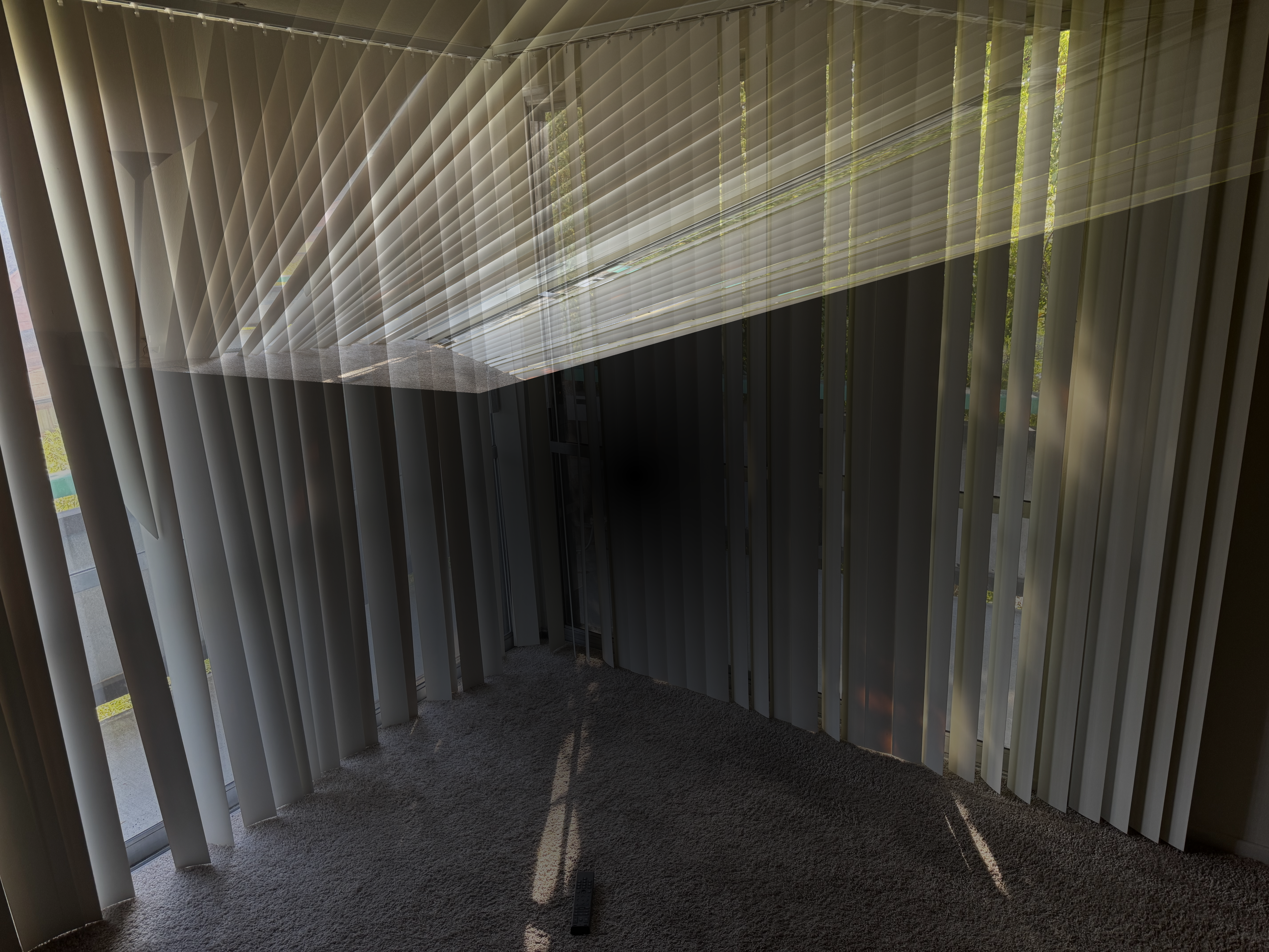
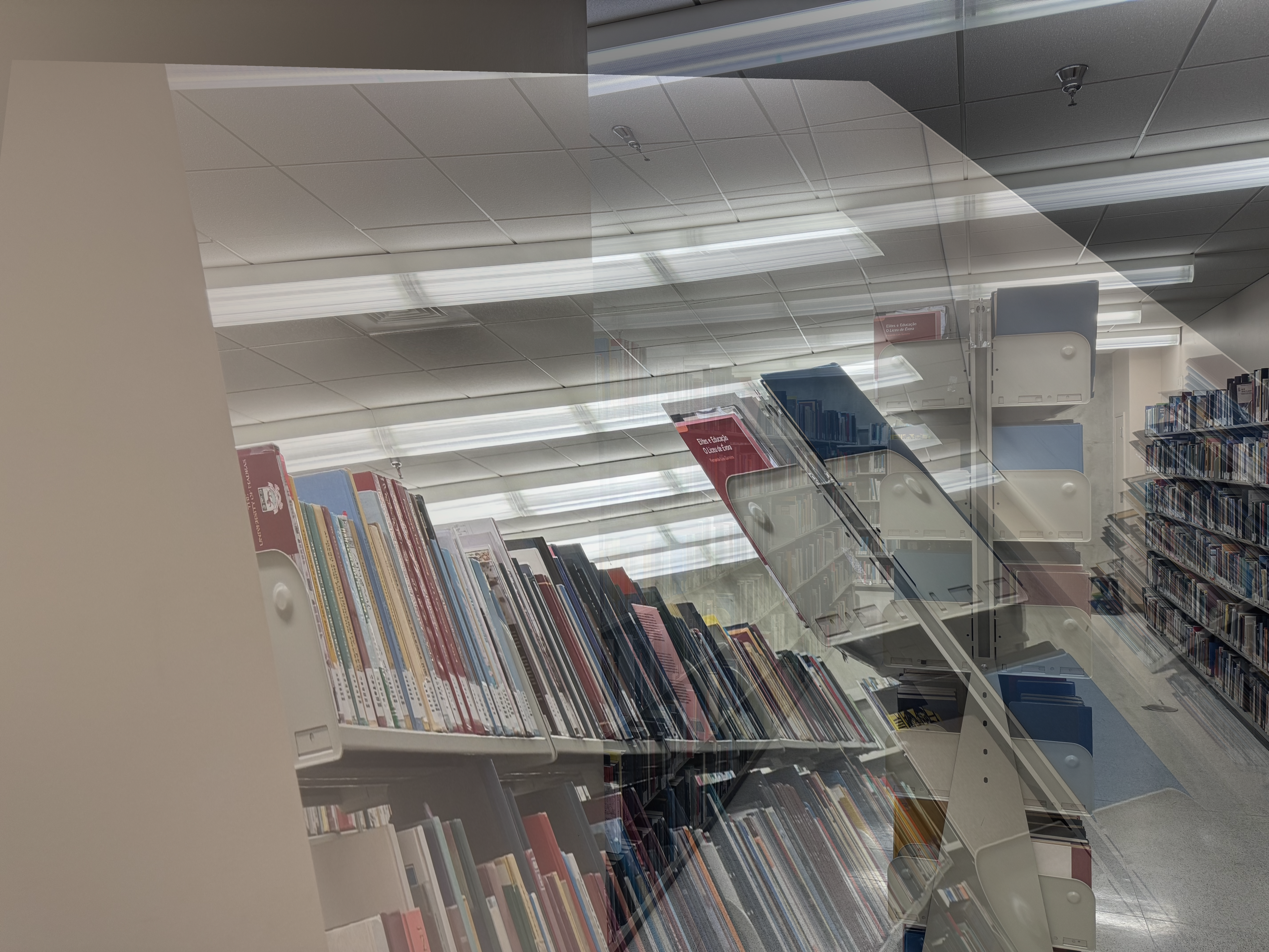
Below are the final mosaics for the three scenes: Tile, Window, and Library. Each mosaic was created by aligning the images using the computed homographies and blending them smoothly with Gaussian-blurred alpha masks.

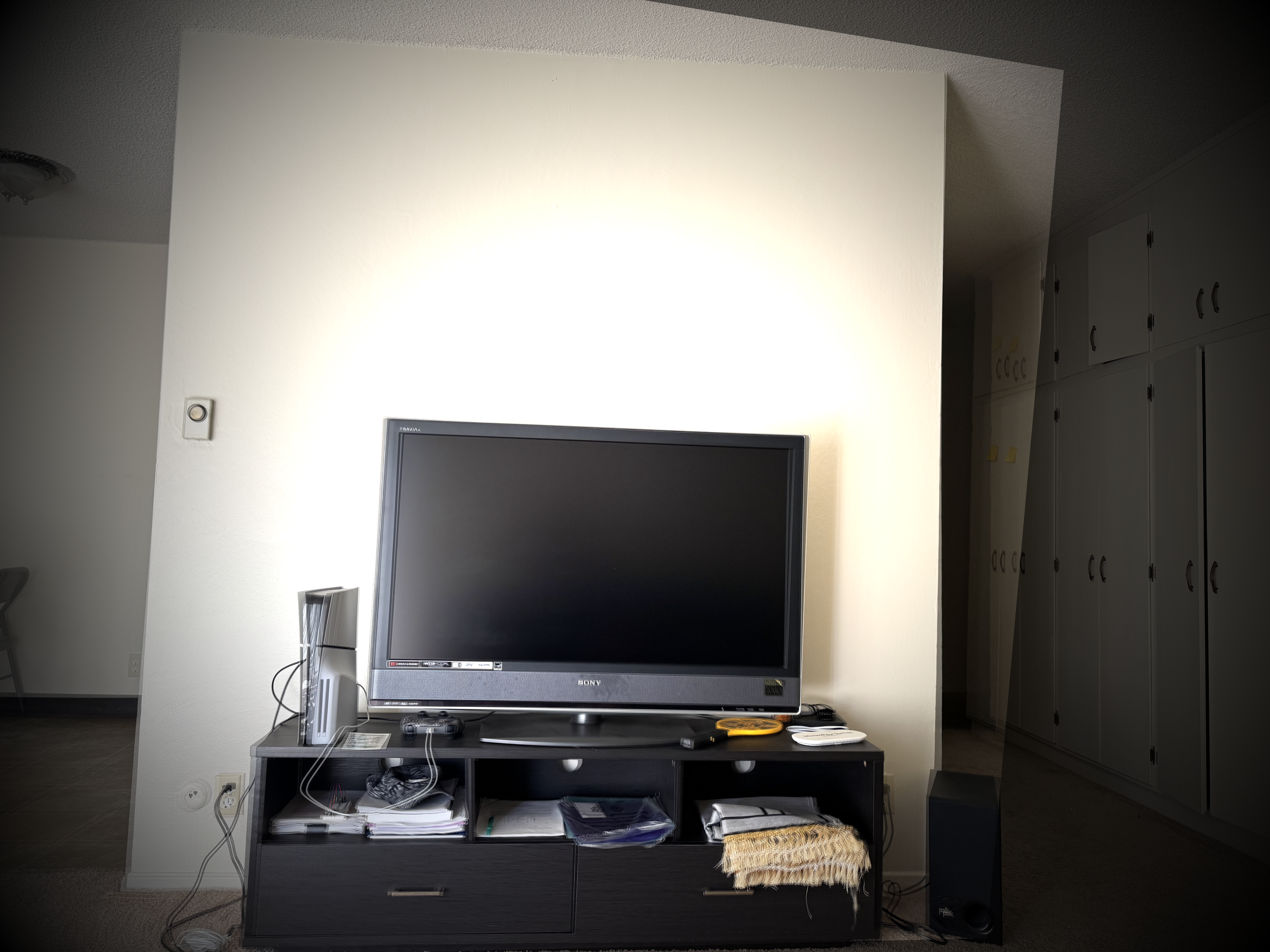
Tile Mosaic

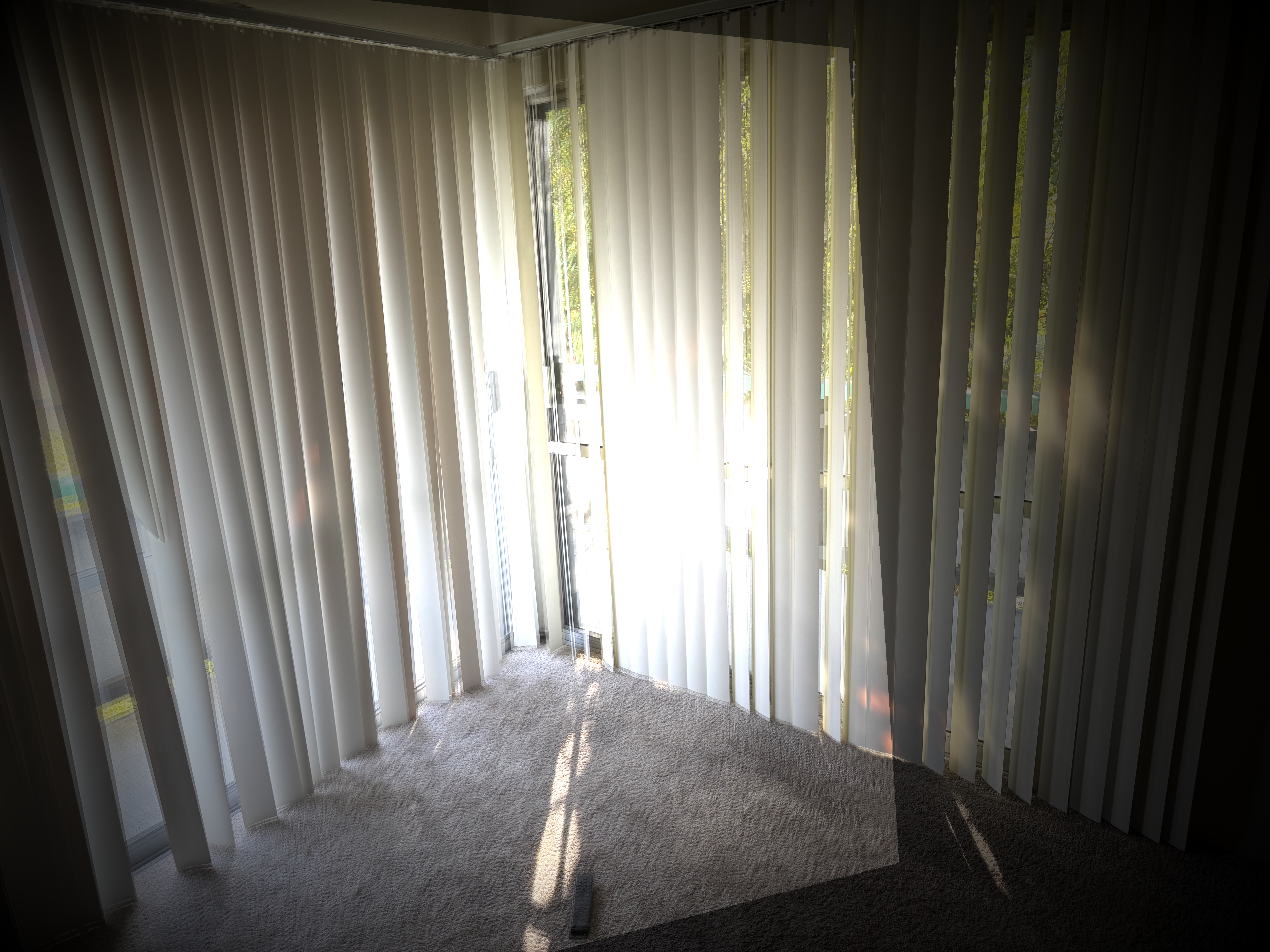
Window Mosaic

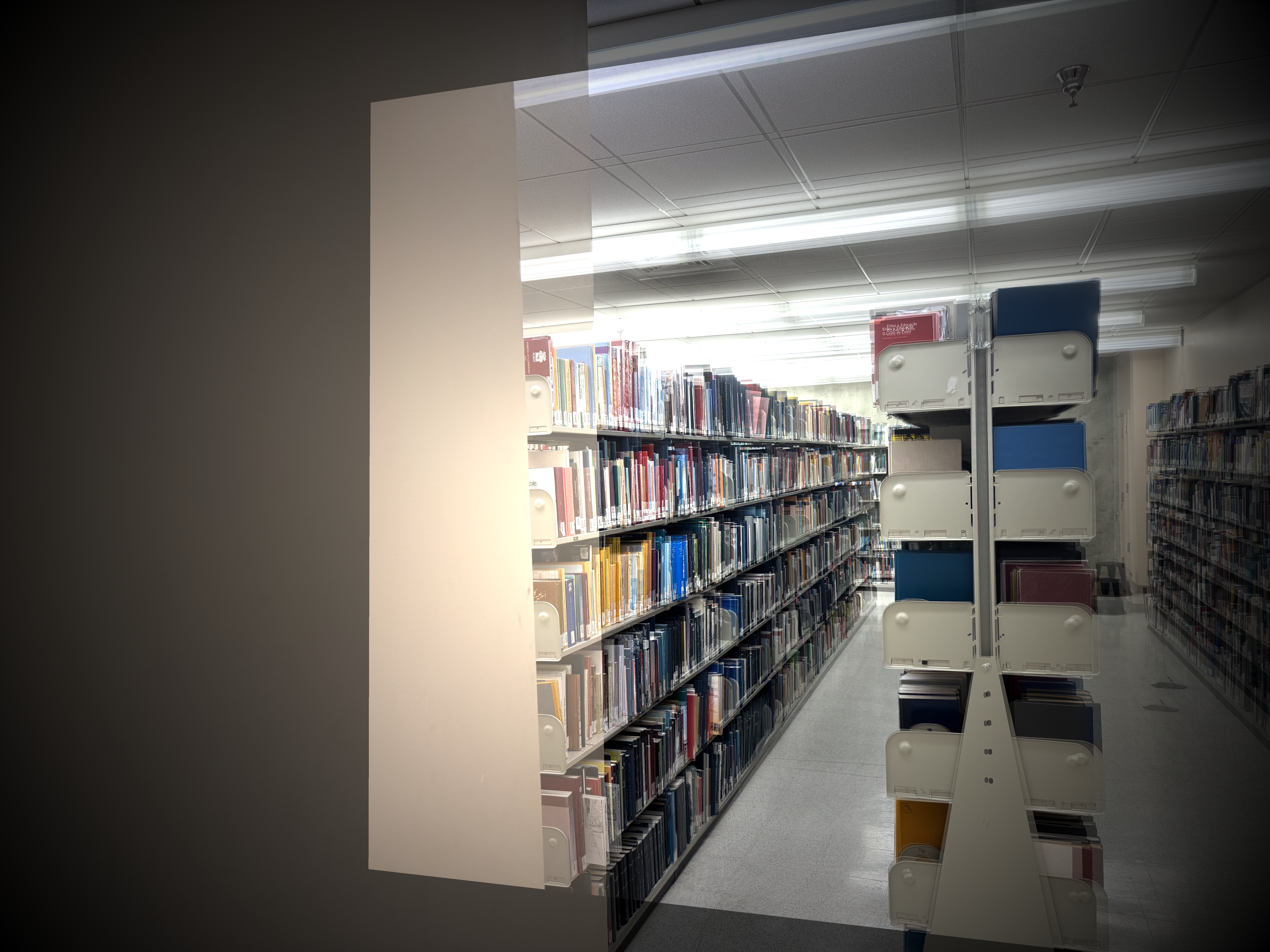
Library Mosaic

Overview - Part B

In Part B, I automated the process using feature detection and matching, robust homography estimation with RANSAC, and generated final mosaics without manual intervention. This approach enhanced accuracy and consistency in creating the mosaics.

Part 5: Feature Detection

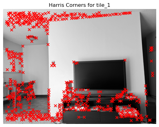
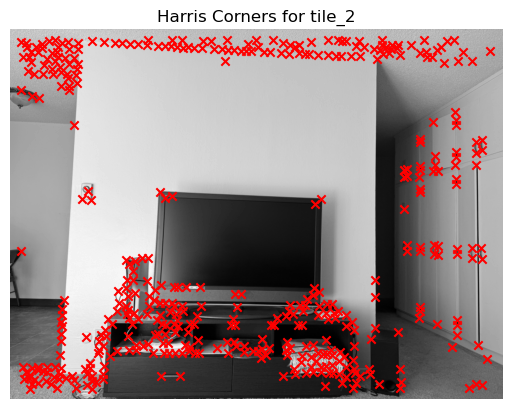
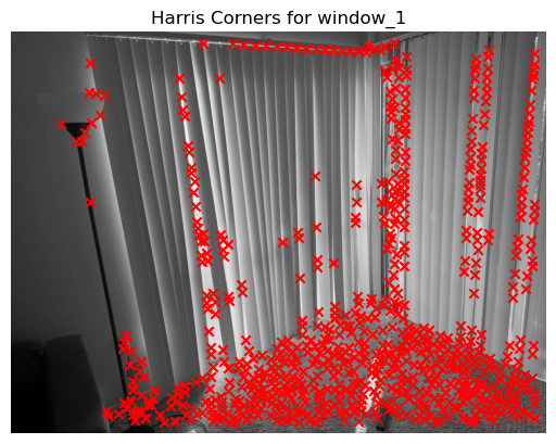
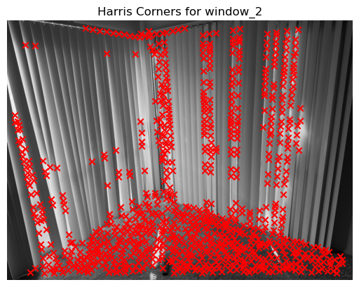
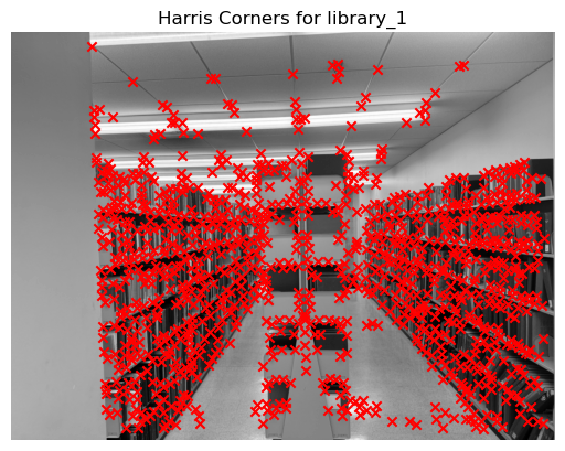
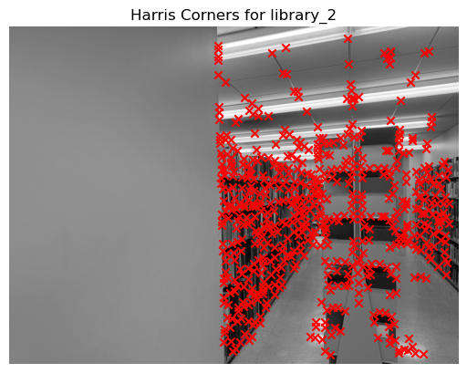
Harris Corner Detection was used to identify points of interest in each image. These feature points were then used in subsequent steps to match corresponding regions between images.

Detected Corners

Tile Area

Window

Library

Part 6: Feature Matching

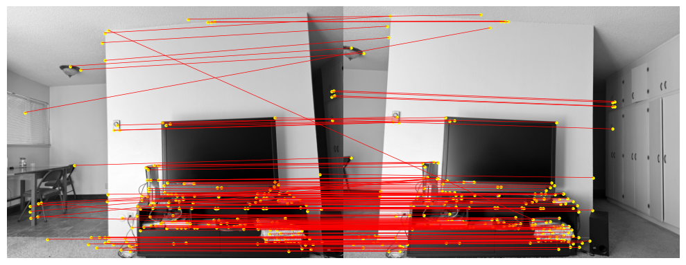
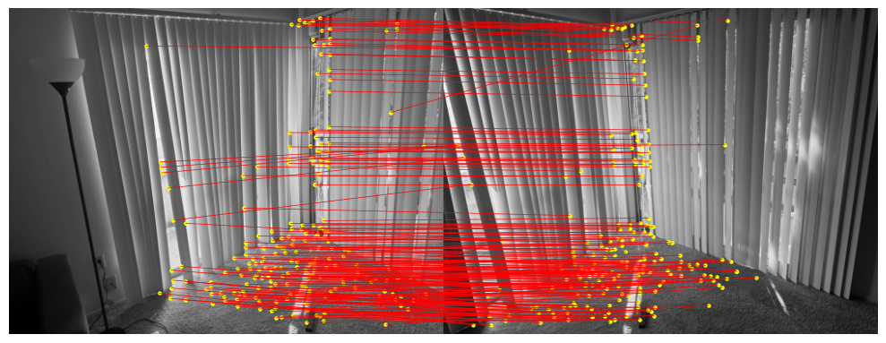
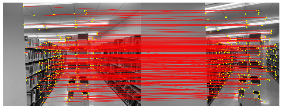
After detecting features, I extracted descriptors and matched them between image pairs. The matches were filtered using a ratio test to retain reliable matches.

Feature Matches

Part 7: RANSAC

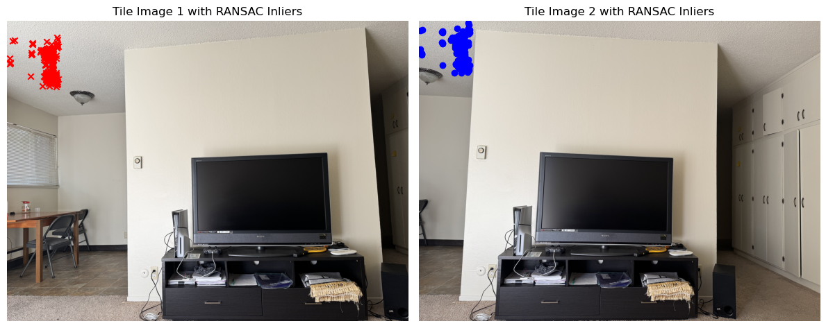
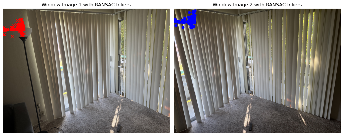
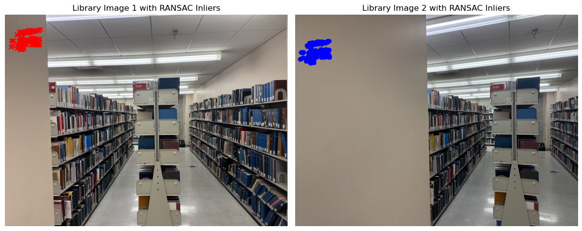
RANSAC was applied to estimate the homography between images while rejecting outliers. This method ensures that only the most consistent feature matches are used to compute the transformation. I made sure to follow the exact steps stated in the lecture slides.

Inliers from RANSAC

Part 8: Automatic Mosaic

Using the homographies estimated through RANSAC, I automatically aligned the images to create seamless mosaics. These results demonstrate the effectiveness of feature-based alignment.

Automatically Generated Mosaics

Conclusion: Coolest Thing I Learned

One of the most fascinating aspects of this project was understanding how homography transformations work and how they enable us to map one plane to another, essentially aligning images captured from different perspectives. It felt like magic to see how a few carefully selected correspondences between images could allow us to compute a transformation matrix that seamlessly aligns and stitches those images together into a panoramic type photo.

Also, implementing the RANSAC algorithm taught me how to make these transformations more robust. RANSAC's ability to automatically identify and exclude outliers from the feature matches,to make sure that only consistent points contribute to the homography estimation, was impressive. It made me appreciate how much of computer vision relies on both precise math and careful handling of imperfect real-world data.